Handling Temperature Distribution and Linear Systems Using MATLAB

MATLAB assignments often involve solving complex problems that require both a solid understanding of the underlying mathematical concepts and proficiency in MATLAB programming. In this blog, we'll explore two types of MATLAB assignment that are common in engineering and applied mathematics: temperature distribution using the explicit method and solving linear systems using the Thomas Algorithm. We'll discuss the step-by-step process to handle these assignments effectively.
Temperature Distribution Using the Explicit Approach
Problem Overview
We will discuss a sample question in your temperature distribution assignment Consider a bar of length 200 mm, where one end is maintained at a temperature of 313.15 K and the other end at 283.15 K. To study the temperature distribution within this bar over time, you need to use the explicit finite difference method.
Step 1: Discretize the Problem

1. Define the Parameters:
- Length of the bar, L=0.2L = 0.2L=0.2 meters
- Number of nodes, N=15N = 15N=15
- Time step, Δt=1 second
- Thermal diffusivity, α\alphaα, a given constant
2. Calculate Spatial Step Size: The spatial step size Δx is calculated as:
.webp)
Here, Δx=0.2/14≈0.0143 meters.
Step 2: Initialize the Temperature Matrix
1. Create a Matrix for Temperature Distribution: Initialize a matrix TTT to store temperature values over time:
L = 0.2; % Length of the bar in meters
N = 15; % Number of nodes
dx = L / (N-1); % Distance between nodes
dt = 1; % Time step in seconds
alpha = 0.01; % Thermal diffusivity, example value
% Temperature matrix (initially zero)
T = zeros(N, 40); % Assuming 40 minutes of simulation
Set Boundary Conditions: The temperature at the ends of the bar is fixed:
T(1, :) = 313.15; % Temperature at the left end
T(end, :) = 283.15; % Temperature at the right end
Step 3: Implement the Explicit Method
1. Apply the Explicit Finite Difference Method: Update the temperature distribution using the formula:
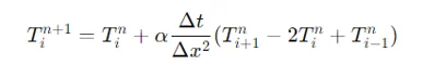
Here's how you can implement it in MATLAB:
for t = 1:40*60 % For each second in 40 minutes
for i = 2:N-1
T(i, t+1) = T(i, t) + alpha * dt / dx^2 * (T(i+1, t) - 2*T(i, t) + T(i-1, t));
end
end
Step 4: Plot the Results
1. Create a Plot for Various Times: Plot temperature distributions at different times (1 min, 3 min, 5 min, 20 min, and 40 min):
time_steps = [1, 3, 5, 20, 40] * 60; % Time in seconds
figure;
hold on;
for t = time_steps
plot(linspace(0, L, N), T(:, t), 'DisplayName', sprintf('%d min', t/60));
end
xlabel('Position (m)');
ylabel('Temperature (K)');
legend;
hold off;
Use Subplots for Different Time Steps: Present temperature distributions with different time steps (1 sec, 5 sec, 20 sec):
time_steps = [1, 5, 20]; % Time steps in seconds
figure;
for i = 1:3
subplot(3,1,i);
T_plot = T(:, time_steps(i));
plot(linspace(0, L, N), T_plot);
title(sprintf('Temperature Distribution at %d seconds', time_steps(i)));
xlabel('Position (m)');
ylabel('Temperature (K)');
end
Observations and Comments
- Analyze how the temperature distribution changes over time and how the bar approaches thermal equilibrium.
- Evaluate the effect of varying time steps on the accuracy and stability of your results.
Linear Systems Using the Thomas Algorithm
Problem Overview
Consider a linear system of equations that needs to be solved using the Thomas Algorithm. The system is:
5x1−x2=5.5
−x1+5x2−x3=5
−x2+5x3−x4=11.5
−x3+5x4=16.5
Step 1: Write the System in Matrix Form
1. Matrix Representation: Convert the system into the tridiagonal matrix form:
.webp)
And

Step 2: Implement the Thomas Algorithm in MATLAB
1. Write the Function: Implement the Thomas Algorithm to solve the tridiagonal system:
function x = tdma(a, b, c, d)
% TDMA algorithm for solving tridiagonal systems
n = length(d);
c_prime = zeros(n-1, 1);
d_prime = zeros(n, 1);
% Forward sweep
c_prime(1) = c(1) / b(1);
d_prime(1) = d(1) / b(1);
for i = 2:n-1
m = 1 / (b(i) - a(i-1) * c_prime(i-1));
c_prime(i) = c(i) * m;
d_prime(i) = (d(i) - a(i-1) * d_prime(i-1)) * m;
end
d_prime(n) = (d(n) - a(n-1) * d_prime(n-1)) / (b(n) - a(n-1) * c_prime(n-1));
% Backward substitution
x = zeros(n, 1);
x(n) = d_prime(n);
for i = n-1:-1:1
x(i) = d_prime(i) - c_prime(i) * x(i+1);
end
end
Test the Function: Apply the function to the provided system:
a = [-1; -1; -1];
b = [5; 5; 5; 5];
c = [-1; -1; -1];
d = [5.5; 5; 11.5; 16.5];
x = tdma(a, b, c, d);
disp('Solution using TDMA:');
disp(x);
Step 3: Compare with MATLAB’s Built-in Solver
1. Use Built-in Solver: Compare the results from the Thomas Algorithm with MATLAB’s built-in solver:
A = diag(b) + diag(a, -1) + diag(c, 1);
x_builtin = A\d';
disp('Solution using MATLAB built-in solver:');
disp(x_builtin);
Observations and Comments
- Examine the solutions obtained from the Thomas Algorithm and MATLAB’s built-in solver.
- Discuss any differences and the accuracy of your implementation.
Conclusion
Solving linear system assignment using MATLAB involves understanding the problem, discretizing the variables, implementing the numerical methods, and interpreting the results. Whether working on heat transfer problems or solving tridiagonal systems, following a systematic approach helps in achieving accurate and reliable solutions. By applying these methods effectively, you can gain valuable insights into the behaviour of physical systems and the efficiency of computational algorithms.