How to Approach MATLAB Assignments Involving Stochastic Differential Equations

MATLAB assignments can often feel daunting, especially when they involve complex topics like stochastic differential equations (SDEs). However, with a systematic approach and a solid understanding of the underlying principles, you can tackle differential equations assignment with confidence. This guide aims to provide a comprehensive approach to solving similar types of MATLAB assignment, focusing on the steps and techniques needed to navigate and solve stochastic differential equations.
Understanding the Problem
The first step in solving any MATLAB assignment is to thoroughly understand the problem statement. This involves identifying the type of differential equation you're dealing with, the initial conditions, and any specific parameters or constraints. It's essential to have a clear grasp of what is required before diving into coding.
Let's break down the approach using a few example problems:
1. Evaluate the steady state covariance matrix for the state of the system:

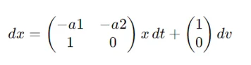
where a1 > 0, a2 > 0 and {v(t),t∈T} is a Wiener process with unit variance parameter.
2. Consider the stochastic differential equation:
dx=Axdt+bdv,
where AAA is a constant n×n matrix, bbb a constant nnn-vector, and {v(t),t∈T} a Wiener process with unit variance parameter. Assume that all eigenvalues of AAA have negative real parts.
3. Show that the steady state covariance of x is given by:
where z is the solution of the differential equation:
dz/dt =Az
with the initial condition z(0)=b.
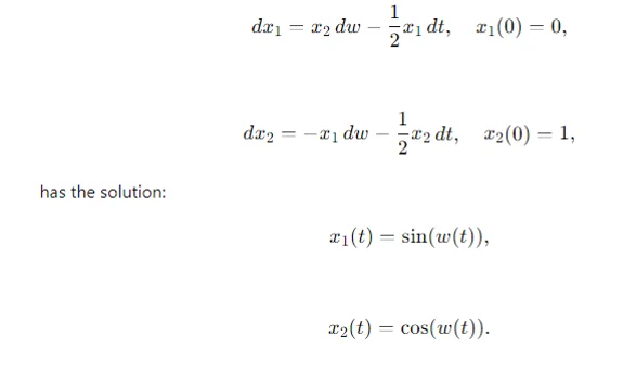
4. Let {w(t),t∈T} be a Wiener process with unit variance parameter. Show that the stochastic differential equation:
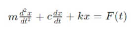
5. A free particle in a liquid can be described by the Langevin equation:
where mmm is the mass, fff the coefficient of viscous friction, and www is the fluctuating force due to collisions with molecules of the liquid. The force www has zero average and covariance function which tends to zero very fast in comparison with m/fm/fm/f. Determine the probability distribution of xxx as a function of time, i.e., determine the mean and covariance matrix of the state of the system.
Breaking Down the Assignment
1. Identify the Type of SDE:
The first step in approaching any SDE problem is to identify the type of differential equation you're dealing with. For example, is it a standard SDE, a Langevin equation, or does it involve specific conditions like steady-state covariance? Recognizing the type of equation will help you decide on the appropriate methods and tools to use in MATLAB.
2. Parameters and Initial Conditions:
Next, clearly note all given parameters, such as matrices, vectors, or initial values. Understanding these parameters is crucial for setting up your problem correctly in MATLAB. For instance, you might have parameters like a1,a2a1, a2a1,a2, matrices AAA, vectors bbb, and initial conditions for the state variables.
3. Required Solution:
Understand what the problem is asking for. Are you required to find a steady-state solution, compute a covariance matrix, or determine a probability distribution? This will guide your approach and the specific MATLAB functions you'll use.
General Steps for Solving SDEs in MATLAB
1. Define the Differential Equation:
Use MATLAB functions like ode45, ode15s, or ode23s for solving ordinary differential equations (ODEs). For stochastic equations, you might need to define the SDE using custom functions. Start by defining the system dynamics using anonymous functions or separate function files.
% Define the system dynamics for a simple ODE
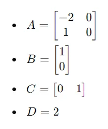
A = [-a1, -a2; 1, 0];
b = [1; 0];
dxdt = @(t, x) A*x + b*randn;
2. Initial Conditions and Parameters:
Define all necessary parameters and initial conditions. This helps in setting up the problem correctly.
Example:
a1 = 1; a2 = 2;
A = [-a1, -a2; 1, 0];
b = [1; 0];
x0 = [0; 1]; % Initial conditions
3. Numerical Solution:
Use appropriate numerical solvers. For SDEs, MATLAB’s built-in functions like sde or custom solvers can be used.
Example:
% Using ode45 for a simple ODE
[t, x] = ode45(@(t, x) A*x + b*randn, [0, 10], x0);
4. Steady-State Analysis:
For steady-state solutions, you might need to solve algebraic equations or use iterative methods to find the covariance matrix.
Example:
% Solve for the steady-state covariance matrix
P_inf = lyap(A, b*b');
5. Plotting and Interpretation:
Visualize the results using MATLAB’s plotting functions to interpret the solutions.
Example:
plot(t, x);
Specific Techniques for Different Types of Problems
1. Evaluating the Steady-State Covariance Matrix:
For a system defined by dx=Ax dt+b dvdx = Ax \, dt + b \, dvdx=Axdt+bdv, find the steady-state covariance matrix using the Lyapunov equation. The MATLAB function lyap is particularly useful for this purpose.
Example:
% Define parameters
A = [-1, -2; 1, 0];
b = [1; 0];
% Calculate the steady-state covariance matrix
P_inf = lyap(A, b*b');
disp('Steady-State Covariance Matrix:');
disp(P_inf);
2. Solving Riccati Equations:
For equations involving Riccati solutions, use MATLAB’s care function to solve for the steady-state covariance. The care function solves the continuous-time algebraic Riccati equation (CARE).
Example:
A = [-1, -2; 1, 0];
B = [1; 0];
Q = eye(2); % Example cost matrix
R = 1;     % Example input cost
% Solve the Riccati equation
[X, L, G] = care(A, B, Q, R);
disp('Solution to Riccati Equation:');
disp(X);
3. Langevin Equation Analysis:
For Langevin-type equations, set up the differential equation and solve for the mean and covariance of the state.
Example:
% Parameters for Langevin equation
m = 1; f = 0.5; kT = 1;
% Define the system dynamics and solve
[t, x] = ode45(@(t, x) [x(2); -f/m*x(2) + sqrt(2*kT/m)*randn], [0, 10], [0; 0]);
% Plot the solution
figure;
plot(t, x(:,1), t, x(:,2));
legend('x', 'dx/dt');
title('Solution of Langevin Equation');
xlabel('Time');
ylabel('State');
General Tips
- Code Structuring: Write modular code with separate functions for defining the system, solving the differential equation, and plotting results. This makes your code more organized and easier to debug.
- aDebugging: Use MATLAB’s debugging tools to step through the code and check for errors. Breakpoints and the disp function are your friends when it comes to understanding what your code is doing at each step.
- Documentation: Comment your code thoroughly to make it easier to understand and maintain. Good documentation helps you and others who might read your code later to understand the purpose and functionality of different parts of your script.
Conclusion
Approaching MATLAB assignments, especially those involving stochastic differential equations, requires a clear understanding of the problem, methodical setup, and appropriate use of MATLAB functions. By following these general steps and techniques, you can tackle similar assignments effectively. Remember, practice is key to mastering MATLAB and solving complex assignments with confidence.
This guide is a starting point, and as you continue to work on MATLAB assignments, you’ll develop your own strategies and techniques. Whether you're evaluating steady-state covariance matrices, solving Riccati equations, or analyzing Langevin equations, the principles outlined here will help you navigate and solve these problems efficiently. Happy coding!