How to Solve Differential Equation Assignments Using MATLAB

Mathematical modeling is an essential part of solving problems in various scientific and engineering fields. Differential equations are widely used to describe dynamic systems that change over time, such as population growth, mechanical systems, electrical circuits, and more. For students studying these systems, solving differential equations can often seem overwhelming, especially when combined with the need to use a tool like MATLAB for simulation and analysis. In this blog, we will walk through a systematic approach to solve your MATLAB assignment related differential equation, from understanding the problem to formulating the equation, solving it, and analyzing the results. This guide is not specific to any one type of problem but provides a general approach that students can apply to various kinds of assignments involving differential equations.
1. Understanding the Problem Statement

Before diving into the solution process, it's essential to fully comprehend the problem at hand. Many assignments will provide a scenario or system that needs to be modeled using a differential equation. A careful reading of the problem will help you understand the type of system involved, the key variables, and how these variables relate to each other. For example, problems may involve:
- Population Growth Models: These problems often involve modeling the population of a species over time using logistic growth or exponential growth models.
- Mechanical Systems: These could involve systems like spring-mass systems, where you need to model the position of a mass connected to a spring.
- Electrical Circuits: Involving RLC circuits (resistor, inductor, capacitor), where you need to model the voltage or charge over time.
- Damping Systems: These involve systems that have forces that resist motion, often modeled as a function of velocity.
When approaching such problems, your goal is usually to:
- Formulate the correct differential equation that describes the system's behavior.
- Identify the appropriate method for solving the differential equation (analytically or numerically).
- Use MATLAB to solve and plot the solution to the differential equation.
- Analyze the solution and interpret the system's behavior over time.
By breaking down the problem into these steps, you will have a clear path to follow and ensure that no part of the assignment is overlooked.
2. Formulating the Differential Equation
The next step after understanding the problem is to formulate the differential equation that represents the system. This is usually the most challenging part for many students, as it requires knowledge of how to model real-world phenomena mathematically. Below are examples of how to approach this step for different types of systems:
a) Population Growth Model
A common example in many assignments is the logistic population model. It models how a population grows in an environment with limited resources. The general form of the logistic growth equation is:
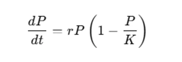
Where:
- P(t) represents the population at time t,
- r is the growth rate,
- K is the carrying capacity (the maximum sustainable population).
In problems where you are given initial conditions (e.g., the population at time t=0t = 0t=0 is 200), you need to substitute these values into the equation to obtain a specific model for your system.
b) Mechanical Systems (Spring-Mass Systems)
Another common scenario is the spring-mass system, where a mass is attached to a spring and subjected to forces such as damping and external forcing. The equation of motion for a damped harmonic oscillator can be written as:
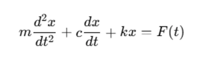
Where:
- x(t) is the displacement of the mass at time t,
- m is the mass,
- c is the damping coefficient,
- k is the spring constant,
- F(t) is an external forcing function.
This equation represents the balance between the forces acting on the mass, including the spring force (proportional to the displacement), the damping force (proportional to velocity), and the external force F(t).
c) Electrical Circuits (RLC Circuits)
In problems involving electrical circuits, such as RLC circuits, the voltage, current, and charge on the components (resistor, inductor, and capacitor) must be related through Kirchhoff’s laws. The charge on the capacitor in an RLC circuit is often governed by the following second-order differential equation:
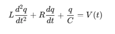
Where:
- q(t) is the charge on the capacitor at time t,
- L is the inductance,
- R is the resistance,
- C is the capacitance,
- V(t) is the voltage source.
This equation reflects the balance of energy in the circuit, where the rate of change of charge is influenced by the inductance, resistance, and the capacitor’s charging behavior.
d) Damped Systems
Damped systems, such as the damped harmonic oscillator or mass-spring-damping systems, are often used in mechanical or electrical engineering problems. The equation for such a system is typically written as:
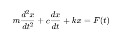
Where:
- x(t) is the position or displacement of the mass at time t,
- m is the mass,
- c is the damping coefficient,
- k is the spring constant,
- F(t) is the external force applied.
This equation can describe systems ranging from simple mechanical oscillations to complex electrical circuits.
3. Choosing the Solution Method
Once you have formulated the differential equation, the next step is to select the appropriate solution technique. Depending on the complexity and type of equation, you have a few options for solving the differential equation.
a) Analytical Solutions
If the differential equation is linear with constant coefficients, you can solve it analytically using various techniques, such as:
- Separation of Variables: This is useful for simple first-order differential equations.
- Integrating Factor: This method is often used for linear first-order differential equations.
- Characteristic Equation: This is used for second-order linear differential equations with constant coefficients.
However, many differential equations encountered in real-world problems are not easily solvable analytically, especially if they involve nonlinear terms or variable coefficients.
b) Numerical Solutions
For more complex equations, numerical methods are often used. MATLAB provides powerful functions for solving differential equations numerically. The most commonly used methods include:
- Euler’s Method: A simple numerical method that approximates the solution by taking small steps forward in time.
- Runge-Kutta Methods: A more accurate method than Euler’s, typically implemented using ode45 in MATLAB.
- MATLAB’s Built-in Functions: MATLAB has several built-in solvers, such as ode45, ode23, and dsolve, that are designed to handle a wide variety of differential equations.
MATLAB’s numerical solvers use time-stepping algorithms to approximate the solution over a specified interval, which is useful when dealing with more complex systems where an analytical solution is not possible.
4. Solving the Differential Equation with MATLAB
Once you have formulated the differential equation and chosen the solution method, MATLAB can help you solve the problem. MATLAB is a powerful tool that provides both symbolic and numerical solutions to differential equations. Here's how you can approach solving differential equations using MATLAB:
a) Symbolic Solutions with dsolve
For simpler differential equations, you can use MATLAB's symbolic toolbox to find an exact solution. Here’s an example of solving a differential equation symbolically:
syms y(t)
Dy = diff(y, t);  % First derivative of y with respect to t
eqn = Dy == 0.1 * y * (1 - y / 800);  % Logistic growth equation
sol = dsolve(eqn, y(0) == 200);  % Solve with initial condition y(0) = 200
disp(sol);
b) Numerical Solutions with ode45
For more complex equations, you can use MATLAB's ode45 function, which is based on the Runge-Kutta method. This function provides numerical solutions for ordinary differential equations (ODEs). For example, solving a logistic growth equation numerically:
% Define the logistic growth equation as a function
function dydt = logistic_growth(t, y)
    r = 0.1;  % Growth rate
    K = 800;  % Carrying capacity
    dydt = r * y * (1 - y / K);  % Logistic growth model
end

% Define initial conditions and time span
y0 = 200;  % Initial population
tspan = [0 100];  % Time range

% Solve the ODE
[t, y] = ode45(@logistic_growth, tspan, y0);

% Plot the solution
figure;
plot(t, y, '-o');
xlabel('Time (years)');
ylabel('Population');
title('Logistic Population Growth');
c) Plotting the Solution
Once you have solved the differential equation, you can visualize the solution using MATLAB’s plotting functions. MATLAB’s plot, fplot, and surf functions can be used to visualize both numerical and symbolic solutions.
figure;
plot(t, y, '-o');  % Plot the population over time
xlabel('Time (years)');
ylabel('Population');
title('Population Growth Over Time');
5. Analyzing the Solution
After obtaining the solution to the differential equation, the next step is to analyze the results. Depending on the problem, you may need to consider different aspects of the solution:
- Long-term Behavior: For population models, you may be interested in the steady-state population, i.e., the population size as time tends to infinity.
- Transient Behavior: For mechanical systems or electrical circuits, you might want to analyze how the system behaves over time before reaching equilibrium.
- Time to Achieve a Specific State: In some problems, you may be asked to determine how long it takes for a system to reach a particular state, such as 95% of the maximum population in a logistic growth model.
You can use MATLAB to perform additional calculations or analyses, such as finding the time it takes to reach a certain threshold, or calculating the steady-state solution.
6. Verifying the Results
It's always a good practice to verify your results to ensure that they are correct. If your assignment requires you to compare numerical and symbolic solutions, you can plot both solutions on the same graph to check for consistency. For example:
This comparison allows you to see how well your numerical solution matches the symbolic one, providing confidence in the accuracy of your results.
Conclusion
Solving MATLAB differential equation assignments involves several key steps: understanding the problem, formulating the differential equation, choosing the right solution method, solving the equation using MATLAB, and analyzing the results. By following a systematic approach, students can effectively tackle complex differential equation problems and gain deeper insights into the behavior of dynamic systems. Remember, MATLAB is a powerful tool that can help you visualize and solve these equations efficiently. Whether you're working with population models, mechanical systems, or electrical circuits, MATLAB offers the necessary functions and capabilities to assist you in solving and understanding these problems. By mastering these steps and utilizing MATLAB effectively, you'll be well-equipped to complete your differential equation assignment with confidence.