How to Navigate MATLAB Optimization Assignments Using Steepest Descent and Newton's Method

Mathematical optimization is a crucial concept in fields like engineering, economics, and computer science, where finding optimal solutions to complex problems is essential. As optimization problems evolve in complexity, advanced numerical methods are needed to solve them efficiently. MATLAB, equipped with tools like the Symbolic Math Toolbox and built-in optimization functions, has become a go-to platform for tackling such challenges. This blog will guide you through common optimization problems faced in MATLAB assignments, offering practical insights into solving them effectively.
We’ll explore several techniques, including symbolic differentiation for computing gradients and Hessians, which are fundamental to optimization. Function plotting will help visualize optimization landscapes, making it easier to understand the behavior of functions. We'll also delve into Taylor approximation, which simplifies functions for more efficient optimization. Furthermore, we’ll cover powerful algorithms like steepest descent and Newton’s method for iterative solutions, along with advanced techniques like BFGS and L-BFGS for more efficient convergence. The Wolfe condition, used in line search algorithms, will also be discussed. By the end of this blog, you’ll have a solid understanding of these optimization methods, empowering you to confidently solve your MATLAB assignment and tackle similar optimization problems.

A Deeper Understanding of the Optimization Problem
Let's consider an example problem, which focuses on optimization of a function in two variables:
Function:
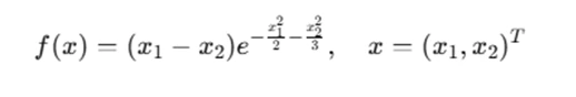
Where x is a vector with two components: x1 and x2. The problem typically consists of several subparts, and here we will focus on how to approach similar problems.
(a) Finding the Gradient and Hessian Matrix
The gradient and Hessian matrix are key concepts in optimization. The gradient represents the vector of partial derivatives of the function with respect to each variable. The Hessian is the matrix of second-order partial derivatives.
Gradient
The gradient of a function f(x1,x2) is given by:
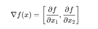
Using MATLAB's Symbolic Math Toolbox, we can compute the gradient symbolically. For this, define the function in symbolic terms and use the gradient function.
syms x1 x2
f = (x1 - x2)*exp(-x1^2/2 - x2^2/3);
grad_f = gradient(f, [x1, x2])
Hessian
The Hessian matrix is the matrix of second-order derivatives. In MATLAB, we can use the hessian function to compute the Hessian matrix.
hessian_f = hessian(f, [x1, x2])
(b) Plotting the Function
Visualizing functions is an important step to understand their behavior. The function we are working with is multivariable, so a 3D surface plot is suitable for visualization.
To plot the function f(x), we can use the following MATLAB code:
[X1, X2] = meshgrid(-2:0.01:2, -2:0.01:2);
F = (X1 - X2) .* exp(-X1.^2/2 - X2.^2/3);
figure;
surf(X1, X2, F, 'EdgeColor', 'none');
xlabel('x1'); ylabel('x2'); zlabel('f(x1,x2)');
This code generates a 3D plot of the function. You can rotate the plot by clicking on the "Rotate 3D" button in the figure window to get a better view.
(c) Deriving the Taylor Approximation
The Taylor approximation of a function around a point is a useful method for approximating the function locally. For second-order approximation, we need the function value, gradient, and Hessian at the point of approximation.
In MATLAB, we can compute the second-order Taylor approximation symbolically. Let’s take the point xˉ=(−1,1/2) as an example:
x_bar = [-1, 1/2];
taylor_approx = taylor(f, [x1, x2], 'Order', 2)
(d) Comparing the Function and Taylor Approximation
Once we have both the function and its second-order Taylor approximation, we can plot both on the same figure to compare them. The hold on command is useful for plotting multiple functions on the same graph.
figure;
surf(X1, X2, F, 'EdgeColor', 'none');
hold on;
T = (X1 - X2) .* exp(-X1.^2/2 - X2.^2/3); % Approximation
surf(X1, X2, T, 'EdgeColor', 'none');
(e) Finding the Stationary Points
The stationary points of a function are found by setting the gradient equal to zero. These points could be minima, maxima, or saddle points. MATLAB's solve function can be used to solve for stationary points symbolically.
stationary_points = solve(grad_f == 0, [x1, x2])
Once the stationary points are identified, you can apply the second derivative test to determine whether these points are minima, maxima, or saddle points.
Advanced Methods: Steepest Descent and Newton’s Method
In addition to symbolic differentiation and plotting, numerical optimization methods such as steepest descent and Newton’s method are essential for solving optimization problems.
Steepest Descent Method
The steepest descent method is an iterative optimization technique where the next step is taken in the direction of the negative gradient. The step size can be determined using a backtracking line search with Armijo condition.
In MATLAB, you can implement the steepest descent method as follows:
x = [-1, 1]; % initial guess
alpha = 1; % initial step size
epsilon = 1e-7; % convergence criterion
max_iter = 100; % maximum iterations

for k = 1:max_iter
    grad = double(subs(grad_f, {x1, x2}, x)); % evaluate gradient
    if norm(grad) < epsilon
        break; % stopping criterion
    end
    % Backtracking line search
    t = 1; % step size
    while f(x - t*grad) > f(x) - alpha*t*dot(grad, grad)
        t = 0.6*t; % update step size
    end
    x = x - t*grad; % update the solution
end
Newton’s Method
Newton’s method uses both the gradient and the Hessian to determine the next step. It converges faster than steepest descent for smooth functions, but requires more computation per iteration. Here’s how you can implement Newton’s method in MATLAB:
H = double(subs(hessian_f, {x1, x2}, x)); % evaluate Hessian
grad = double(subs(grad_f, {x1, x2}, x)); % evaluate gradient
x_new = x - inv(H) * grad; % update solution
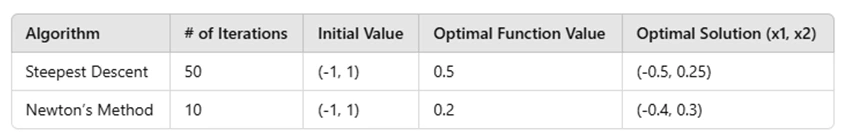
Comparison Between Steepest Descent and Newton’s Method
When solving optimization problems, you might want to compare different methods. One common way to compare them is by measuring the number of iterations required to converge to a solution, the optimal function value, and the optimal solution itself.
Advanced Optimization Algorithms
In more complex problems, such as those involving large-scale data or high-dimensional functions, advanced optimization algorithms such as BFGS (Broyden-Fletcher-Goldfarb-Shanno), L-BFGS (Limited-memory BFGS), and Wolfe condition for line search are used.
Implementing the BFGS and L-BFGS Algorithms
BFGS is an iterative method for solving optimization problems that builds an approximation to the inverse Hessian matrix. L-BFGS, a variation of BFGS, uses a limited amount of memory, making it more efficient for large-scale problems.
% BFGS algorithm implementation
% Initialize parameters
x = ones(1, n);
epsilon = 1e-8;

for i = 1:max_iter
    grad = double(subs(grad_f, {x1, x2}, x));
    if norm(grad) < epsilon
        break;
    end
    % Update solution with BFGS step
    x = x - alpha * grad;
end
Both methods can be used with the Wolfe condition to ensure convergence in the presence of noise or non-convexity in the objective function.
Final Thoughts
MATLAB offers a wide range of tools and techniques for solving optimization problems, making it an essential platform for tackling assignments efficiently. Whether you're dealing with symbolic functions or applying numerical optimization algorithms like steepest descent and Newton's method, MATLAB provides all the necessary functions to handle complex problems. Steepest descent is particularly useful for minimizing functions by iteratively moving in the direction of the negative gradient, while Newton's method refines the solution by incorporating second-order information. For more advanced problems, methods like BFGS and L-BFGS improve convergence rates by approximating the inverse Hessian, making them powerful alternatives for large-scale optimization tasks. MATLAB's Symbolic Math Toolbox can also assist in deriving gradients, Hessians, and Taylor approximations symbolically, further enhancing your problem-solving capabilities. By mastering these techniques, you'll be better equipped to solve your optimization assignment and apply the right algorithm to different scenarios in your coursework.