How to Approach Robotics and Mechanical Assignments Using MATLAB and Control Systems

Tackling robotics and mechanical system assignments can often feel overwhelming due to the complexity of simulations, mathematical models, and control systems involved. However, MATLAB provides a comprehensive suite of tools that simplifies the process, especially when it comes to robotic system modeling, control, and simulation. By breaking down the problem into manageable steps, MATLAB allows students to model, simulate, and control robotic systems with ease.
The approach begins with modeling the system using Denavit-Hartenberg parameters to define joint positions and calculate transformations. MATLAB’s built-in functions can be used to verify these calculations, ensuring accuracy. Once the system is modeled, students can simulate the kinematics and dynamics of the robotic arm or mechanical system, allowing them to analyze movement and behavior under different conditions. Simscape Multibody is particularly useful for simulating multibody systems and understanding the interactions between components. Control systems, such as PID controllers, can then be implemented to refine the system’s performance, ensuring precise motion and stability. Additionally, MATLAB’s flexibility allows for the integration of more advanced features like flexible body modeling and motor simulations. By following this structured approach, students can solve their robotics assignment and mechanical system effectively, gaining a deeper understanding of both the theoretical and practical aspects of robotics

Step 1: Modeling the System Using Denavit-Hartenberg Parameters
One of the first and most important tasks in any robotic assignment is modeling the geometry of the system. In this step, we use Denavit-Hartenberg (DH) parameters, which are a systematic way to represent the relationship between different joints and links in a robotic arm. The DH parameters define how the coordinate system of one joint is transformed into the next, and they are the backbone of robotic kinematics.
What are Denavit-Hartenberg Parameters?
The Denavit-Hartenberg method is based on four key parameters:
- θ (theta): Joint angle for revolute joints, which defines the rotation around the z-axis.
- d: The offset along the previous z-axis to the common normal, used for prismatic joints.
- a: The distance between the z-axes along the common normal, representing the length of the link.
- α (alpha): The angle between the z-axes of two consecutive joints.
By defining these parameters, you can derive the transformation matrix that represents the relationship between two consecutive coordinate frames in your robotic arm. This matrix allows you to calculate the position and orientation of each joint and link in the system.
How to Approach Modeling with DH Parameters
- Step 1: Identify the joints and links in the system. For example, in a robotic arm, the joints could be revolute or prismatic, and each link would be a rigid body connecting two joints.
- Step 2: For each joint, define the DH parameters—θ, d, a, and α—based on the geometry of the arm.
- Step 3: Use the DH parameters to build the transformation matrices, which will allow you to calculate the position of the arm when all the joint variables are set to zero.
Step 2 Performing Structural Calculations for Robotic Arms
For assignments that involve physical modeling of robotic arms, structural calculations are often needed. These calculations might include determining the bending stress and selecting the appropriate material for the links of the robotic arm. This process ensures the structural integrity of the system under loading conditions.
Bending Stress Calculation
One of the primary calculations when dealing with robotic arms involves determining the bending stress on the links. If the links are beams under load, such as an outstretched robotic arm holding a payload, the bending stress formula is crucial:
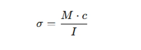
Where:
- σ is the bending stress,
- M is the bending moment,
- c is the distance from the neutral axis to the outermost fiber,
- I is the moment of inertia.
This formula allows you to determine the maximum stress the link will experience, which is essential for choosing the right material and ensuring the system will operate safely under real-world conditions.
How to Approach Structural Calculations
- Step 1: Identify the loads on the robotic arm, such as the payload it will be carrying.
- Step 2: Use beam theory to calculate the bending stress in the arm’s links. You’ll also need to calculate the moment of inertia of the beam’s cross-section.
- Step 3: Choose a material for the links, taking into account its maximum allowable stress and the safety factor required for dynamic loading.
By following these calculations, you’ll ensure that your robotic arm can handle the payload without failure while maintaining structural integrity.
Step 3 Simulating the Robot with Simscape Multibody
After modeling and defining the system’s geometry and materials, the next step is simulation. MATLAB's Simscape Multibody is an ideal tool for simulating the motion of robotic systems. It allows you to create 3D models of your system and analyze how the robotic arm moves under different conditions.
Setting up the Simulation
- Step 1: Define the robot’s links and joints in Simscape. You can model each part as a rigid body or use more complex flexible models, depending on the requirements of your assignment.
- Step 2: Set initial conditions for the robot’s configuration. For example, if the assignment requires simulating the robot with both arms downwards, set this as the home position.
- Step 3: Specify the input motions for each joint. For instance, you might drive the joint angles using a sinusoidal profile to move the arm to a desired position.
Using Simscape for Multibody Simulation
Simscape Multibody provides a powerful environment for simulating the movement and forces acting on the robotic arm. You can model each joint as a revolute joint and input the motion profiles to see how the arm moves and interacts with the payload.
Step 4: Implementing Control Systems with PID Controllers
For robotics assignments, control systems are often required to ensure the arm moves as intended, reducing errors and improving accuracy. One of the most common control strategies is the PID controller, which adjusts the system’s behavior based on the difference between the desired and actual positions.
How to Implement a PID Controller
- Step 1: Begin by tuning the Proportional (P) term to reduce the initial position error.
- Step 2: Add the Integral (I) term to eliminate any steady-state error that may accumulate over time.
- Step 3: Add the Derivative (D) term to stabilize the system and minimize oscillations.
- Step 4: Use MATLAB’s Simulink to build a PID control system and implement it in your robot’s simulation.
By tuning the PID controller parameters, you can achieve smooth and accurate motion, ensuring that the robotic arm reaches its desired position without overshooting or oscillating.
Step 5: Analyzing Flexible Bodies in Simscape
Many assignments also require you to model flexible bodies, especially if the robot arm includes long links or beams. The flexibility of these bodies can have a significant impact on the performance of the system, so it’s essential to evaluate how the flexibility affects the arm’s motion.
Simulating Flexible Bodies
- Step 1: Define the material properties of the flexible beams, including density, Young’s modulus, and Poisson’s ratio.
- Step 2: Use the flexible body model in Simscape to replace the rigid bodies with flexible ones.
- Step 3: Run the simulation and compare the results with the rigid-body model to evaluate how the flexibility affects the robot's performance.
Step 6: Evaluating System Performance and Documenting Results
Once the simulation and control systems are in place, you need to evaluate the performance of the robotic system. This includes analyzing the torque at each joint, the position of the payload, and the impact of flexible bodies on system performance.
Analyzing the Results
- Step 1: Measure the torques at each joint and the joint positions over time.
- Step 2: Compare the performance with and without the PID controller to see how well it reduces errors.
- Step 3: Analyze the differences between the rigid and flexible body models, particularly in terms of the payload position error and overall system behavior.
By comparing these different scenarios, you can understand the importance of flexibility and control in the robotic system’s performance.
Conclusion
Solving complex robotics and mechanical system assignments involves understanding the system’s geometry, performing structural and kinematic calculations, modeling the system in MATLAB, and implementing control systems to ensure smooth and accurate motion. By following the steps outlined in this blog—modeling with Denavit - Hartenberg parameters, performing stress calculations, simulating the system with Simscape, implementing PID control, and evaluating flexible bodies, you can complete your control system assignment with confidence. The key is to break down the tasks step by step, ensuring a clear understanding of the concepts and to solve their Matlab assignment related to robotics and mechanical system problem effectively. By leveraging MATLAB and Simscape Multibody, students can gain valuable insights into the behavior of robotic systems and develop practical skills in control systems, simulation, and engineering analysis.