How to Approach MATLAB Assignments on Probability Density Functions (PDFs)

Probability and statistics play a crucial role in mathematics, engineering, and data science. Many MATLAB assignments require students to analyze probability density functions (PDFs), compute statistical measures, and visualize distributions. Understanding these concepts and using the right MATLAB functions effectively is essential for solving such assignments efficiently.
This guide provides a structured approach to handling probability and statistics assignments in MATLAB. Instead of focusing on a specific problem, it outlines general techniques applicable to similar assignments. The process begins with defining the probability density function and ensuring it satisfies the normalization condition. From there, students can compute key statistical properties such as the mean, variance, and standard deviation. The cumulative distribution function (CDF) helps in determining probabilities and visualizing the distribution.

For assignments involving joint distributions, finding marginal distributions and correlation coefficients provides deeper insights into the relationships between variables. MATLAB’s symbolic and numerical tools simplify these computations, making it easier to analyze and interpret probability distributions. By following this structured approach, students can confidently solve their MATLAB assignment related to probability and statistics, improving both their problem-solving skills and conceptual understanding of statistical analysis.
Understanding Probability Density Functions (PDFs)
A probability density function (PDF) describes the likelihood of a continuous random variable taking specific values within a given range. It must satisfy two key properties: it is always non-negative, and its total integral over all possible values equals one. The PDF does not give direct probabilities for individual points but rather represents the density of probabilities over an interval. By integrating the PDF over a given range, we obtain the probability that the variable falls within that range. PDFs are widely used in probability and statistics to model real-world data and analyze distributions in fields like engineering and data science. The key properties of a PDF include:
- Non-Negativity: The PDF must always be non-negative for all values of x.
- Normalization Condition: The total probability over all possible values must sum to 1:
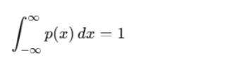
When given a PDF with an unknown parameter, you can determine its value by ensuring that the integral over its range equals 1.
Example in MATLAB
Consider a PDF:
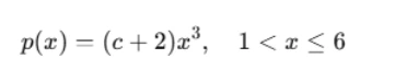
To find the unknown parameter ccc, we solve:
syms x c
pdf = (c + 2) * x^3;
eqn = int(pdf, x, 1, 6) == 1;
c_value = solve(eqn, c);
disp(c_value);
This will return the value of c that satisfies the normalization condition.
Finding the Mean and Variance of a Random Variable
Finding the mean and variance of a random variable is essential for understanding its distribution and behavior. The mean (expected value) represents the average outcome and is calculated by integrating the product of the variable and its probability density function (PDF). The variance measures how much the values deviate from the mean, providing insight into the spread of the distribution. A higher variance indicates greater dispersion, while a lower variance suggests values are closely clustered around the mean. These statistical measures are crucial in probability theory, helping in data analysis, decision-making, and predictive modeling across various fields like engineering and finance.Once the PDF is fully defined, we can compute important statistical measures:
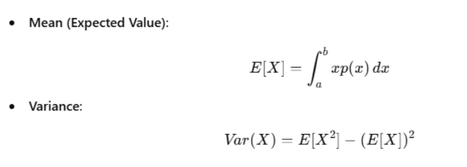
The standard deviation is simply the square root of the variance.
Example MATLAB Code
E_X = int(x * pdf, x, 1, 6);
E_X2 = int(x^2 * pdf, x, 1, 6);
Variance = E_X2 - E_X^2;
disp([E_X, Variance]);
This will return the expected value and variance of X.
Finding the Cumulative Distribution Function (CDF)
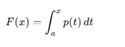
The cumulative distribution function (CDF) provides a comprehensive way to understand the probability distribution of a random variable. It represents the probability that the variable takes a value less than or equal to a given point. Mathematically, the CDF is obtained by integrating the probability density function (PDF) over the given range. The CDF is always non-decreasing and ranges from 0 to 1. It is useful for calculating probabilities over intervals, determining median values, and analyzing the overall behavior of a distribution. In MATLAB, the CDF can be computed symbolically or numerically and visualized using plotting functions for better interpretation. The cumulative distribution function (CDF) gives the probability that the random variable takes a value less than or equal to x:
To plot the CDF in MATLAB, integrate the PDF and use fplot:
F_x = int(pdf, x, 1, x);
fplot(F_x, [1,6]);
xlabel('x');
ylabel('F(x)');
title('Cumulative Distribution Function');
grid on;
This will generate a plot showing how probability accumulates over the range of x.
Computing Probabilities for Specific Ranges
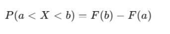
Computing probabilities for specific ranges helps in determining the likelihood of a random variable falling within a given interval. This is done by integrating the probability density function (PDF) over the desired range. The cumulative distribution function (CDF) can also be used by finding the difference between its values at the given points. MATLAB provides functions for numerical integration and built-in statistical tools to compute probabilities efficiently. This process is crucial in real-world applications like risk assessment, reliability analysis, and decision-making in various fields. To find the probability that X falls within a specific range, use the CDF:
In MATLAB, this is implemented as:
P_value = subs(F_x, x, 4) - subs(F_x, x, 3);
disp(P_value);
This calculation provides the probability that X lies between 3 and 4.
Finding the Mode and Median
Finding the mode and median of a random variable provides valuable insights into its distribution. The mode is the value where the probability density function (PDF) reaches its maximum, indicating the most likely outcome. It is found by solving for the critical points of the PDF. The median is the value that divides the distribution into two equal halves, meaning the cumulative distribution function (CDF) at the median equals 0.5. MATLAB’s symbolic and numerical tools make it easier to compute these measures and analyze probability distributions effectively.
- Mode: The mode of a continuous probability distribution is the value of x where p(x) reaches its maximum.
- Median: The median is the value xmx where F(xm)=0.5F.
MATLAB Implementation
mode_value = solve(diff(pdf, x) == 0, x);
median_value = solve(F_x == 0.5, x);
disp([mode_value, median_value]);
This will compute the mode and median of the distribution.
Working with Two-Dimensional Probability Distributions
Two-dimensional probability distributions describe the relationship between two random variables and are represented by a joint probability density function (PDF). This function must satisfy the normalization condition, ensuring the total probability equals one. To analyze such distributions, we compute marginal distributions by integrating out one variable, providing insights into individual behaviors. The correlation coefficient measures the strength and direction of the relationship between the variables. MATLAB offers powerful tools for visualizing joint distributions, computing probabilities, and analyzing dependencies. Understanding two-dimensional distributions is crucial in fields like machine learning, finance, and engineering, where multiple variables interact in complex ways. When dealing with a joint probability distribution, the given function represents the probability of two random variables, X and Y, occurring together.
Key Steps for Solving Joint Distribution Problems
- Find the Normalizing Constant: Ensure that the total probability equals 1.
- Find Marginal PDFs: Obtain the individual distributions of X and Y.
- Compute Mean, Variance, and Standard Deviation for X and Y.
- Find the Correlation Coefficient: Measure the dependence between X and Y.
Example MATLAB Code for Joint PDF
Consider the joint PDF:
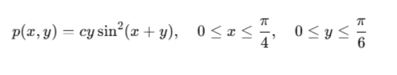
To find the unknown parameter c:
syms x y c
pdf_xy = c * y * sin(x+y)^2;
eqn = int(int(pdf_xy, x, 0, pi/4), y, 0, pi/6) == 1;
c_value = solve(eqn, c);
disp(c_value);
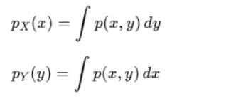
Finding Marginal Distributions
The marginal distributions of X and Y are found by integrating out the other variable:
Example MATLAB Code
p_X = int(pdf_xy, y, 0, pi/6);
p_Y = int(pdf_xy, x, 0, pi/4);
disp([p_X, p_Y]);
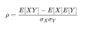
Finding Correlation Coefficient
The correlation coefficient measures the strength and direction of the relationship between two random variables. It is calculated using the covariance and standard deviations of the variables. A value close to 1 or -1 indicates a strong relationship, while a value near 0 suggests little to no correlation. In MATLAB, it can be computed using built-in statistical functions for efficient analysis. The correlation coefficient measures how strongly X and Y are related:
MATLAB Code for Correlation
E_XY = int(int(x*y*pdf_xy, x, 0, pi/4), y, 0, pi/6);
E_X = int(x*p_X, x, 0, pi/4);
E_Y = int(y*p_Y, y, 0, pi/6);
Variance_X = int((x - E_X)^2 * p_X, x, 0, pi/4);
Variance_Y = int((y - E_Y)^2 * p_Y, y, 0, pi/6);
Correlation = (E_XY - E_X * E_Y) / sqrt(Variance_X * Variance_Y);
disp(Correlation);
Conclusion
In conclusion, solving probability and statistics assignments in MATLAB requires a systematic approach that includes defining the probability density function, ensuring it is properly normalized, and computing key statistical properties such as the mean, variance, and standard deviation. Understanding the cumulative distribution function allows for probability calculations and visual representation of data distributions. Additionally, finding the mode and median helps in interpreting the distribution characteristics. When dealing with joint distributions, computing marginal distributions and correlation coefficients provides deeper insights into the relationship between random variables. MATLAB's powerful symbolic and numerical tools make these computations efficient and allow for clear visualization of results. By following this structured method, students can confidently tackle a wide range of probability and statistics assignments, gaining a better understanding of key concepts and their applications.