Understanding Forced Vibration, Lumped-Mass Models, and Modal Analysis in MATLAB

Vibration analysis is a fundamental aspect of engineering and physics, playing a critical role in the design and analysis of mechanical systems. For students studying these disciplines, MATLAB often becomes an essential tool for solving vibration-related assignments. These tasks require not only a strong understanding of the theoretical concepts but also the ability to translate these concepts into practical, computational solutions. This blog will walk you through the key aspects of vibration analysis and provide guidance on how to effectively solve your Matlab assignment.
Understanding the Problem Statement
The first and most crucial step in any assignment is to thoroughly understand the problem statement. Whether the assignment involves forced vibration response, modal analysis, or impulse response, a clear understanding of what is being asked is essential for success. Forced Vibration assignment typically combine theoretical derivations with computational analysis. They may require you to model a physical system, derive equations of motion, and solve these equations using MATLAB. This combination can be daunting, but breaking down the problem into manageable steps can help.
Key Questions to Ask:

- What physical system is being modeled?
- What are the key parameters (e.g., mass, stiffness, damping)?
- What type of vibration is being analyzed (free, forced, damped, undamped)?
- Are there any specific outputs required, such as frequency response or time-domain analysis?
By answering these questions, you can gain a clearer understanding of the problem and start planning your approach.
Forced Vibration Response Over Frequency and Damping Ratio
Forced vibration occurs when an external force drives a system. The system's response depends on the frequency of the external force and the damping ratio of the system. The damping ratio determines whether the system is underdamped (oscillatory response), critically damped (fastest non-oscillatory response), or overdamped (slow non-oscillatory response).
Setting Up the Differential Equations
The starting point for analyzing forced vibration is setting up the differential equation that governs the system's motion. For a simple mass-spring-damper system, the equation might look like:
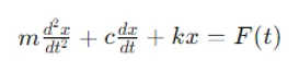
Where:
- mmm is the mass,
- ccc is the damping coefficient,
- kkk is the stiffness,
- xxx is the displacement,
- F(t)F(t)F(t) is the external force as a function of time.
Using MATLAB’s ode45 Function
MATLAB’s ode45 solver is ideal for solving ordinary differential equations (ODEs) numerically. The ode45 function is based on an adaptive step-size Runge-Kutta method, making it well-suited for most ODEs.
Example:
Suppose you need to find the response of a mass-spring-damper system to a harmonic force F(t)=F0cos(ωt)F(t) = F_0 \cos(\omega t)F(t)=F0cos(ωt). You can set up the ODE in MATLAB as follows:
m = 1; % Mass
c = 0.1; % Damping coefficient
k = 10; % Stiffness
F0 = 1; % Amplitude of the external force
omega = 2; % Frequency of the external force
% Define the ODE as a function handle
odefun = @(t, x) [x(2); (F0*cos(omega*t) - c*x(2) - k*x(1))/m];
% Solve the ODE using ode45
[t, x] = ode45(odefun, [0 10], [0 0]);
% Plot the displacement response
plot(t, x(:,1));
xlabel('Time (s)');
ylabel('Displacement (m)');
title('Forced Vibration Response');
Analyzing the Frequency Response
The frequency response of the system shows how it responds to different frequencies of the external force. MATLAB’s Fast Fourier Transform (FFT) function can help analyze this response.
Example:
Y = fft(x(:,1));
f = (0:length(Y)-1)*Fs/length(Y); % Frequency vector
plot(f, abs(Y));
xlabel('Frequency (Hz)');
ylabel('Magnitude');
title('Frequency Response');
In this example, Fs is the sampling frequency, and the fft function is used to compute the frequency spectrum of the displacement response.
Lumped-Mass Model for Beam
When analyzing a beam, it’s common to model it as a series of lumped masses connected by springs. This simplification allows you to use matrix methods to analyze the system.
Dividing the Beam into Segments
Start by dividing the beam into equal segments. Each segment is represented by a lumped mass connected to its neighbors by springs. This transforms the continuous beam into a discrete system.
Deriving the Mass and Stiffness Matrices
The next step is to derive the mass and stiffness matrices for the system. The mass matrix represents the distribution of mass in the system, while the stiffness matrix represents the spring constants.
Example:
If the beam is divided into n segments, the mass matrix M and stiffness matrix K might look like:
M = diag([m1, m2, m3, ..., mn]);
K = [k1 -k1  0  ...  0;
-k1 k1+k2 -k2 ...  0;
0 -k2 k2+k3 ...  0;
...
Modal Analysis
Modal analysis is used to determine the natural frequencies and mode shapes of the system. This can be done by solving the eigenvalue problem for the system matrices.
Example:
[eigenvectors, eigenvalues] = eig(K, M);
natural_frequencies = sqrt(diag(eigenvalues));
The eig function computes the eigenvalues and eigenvectors of the system, where the square root of the eigenvalues gives the natural frequencies.
Visualization
Visualizing the mode shapes helps understand how the beam will deform at each natural frequency. MATLAB’s plotting functions can be used for this purpose.
Example:
for i = 1:length(natural_frequencies)
plot(eigenvectors(:,i));
hold on;
end
xlabel('Segment');
ylabel('Mode Shape');
title('Mode Shapes of the Beam');
legend('Mode 1', 'Mode 2', ..., 'Mode n');
This plot shows how each segment of the beam displaces at different natural frequencies.
Modelling Using Lagrange’s Equation
Lagrange’s equation is a powerful method for deriving the equations of motion for a system. It is especially useful for systems with multiple degrees of freedom, such as a vibrating beam.
Identifying Generalized Coordinates
The first step in using Lagrange’s equation is to identify the generalized coordinates. These are the variables that describe the configuration of the system. For a vibrating beam, the generalized coordinates might be the vertical displacements of the lumped masses.
Computing Kinetic and Potential Energy
Next, write down the expressions for the kinetic and potential energy of the system.
- Kinetic Energy (T): The kinetic energy is the sum of the kinetic energies of all the masses.
- Potential Energy (V): The potential energy is the sum of the elastic potential energies stored in the springs.
Example:
syms x1 x2 x3 ... xn dx1 dx2 dx3 ... dxn;
T = 0.5*m1*dx1^2 + 0.5*m2*dx2^2 + ... + 0.5*mn*dxn^2;
V = 0.5*k1*(x2-x1)^2 + 0.5*k2*(x3-x2)^2 + ... + 0.5*kn*(xn-xn-1)^2;
Deriving the Equations of Motion
Apply Lagrange’s equation, which states:
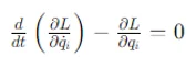
Where L=T−VL = T - VL=T−V is the Lagrangian of the system.
Example:
L = T - V;
eqns = diff(diff(L, dx1), t) - diff(L, x1) == 0;
This symbolic approach in MATLAB allows you to derive the equations of motion for the system.
Modal Analysis
Modal analysis is crucial for understanding how a system behaves at its natural frequencies. It involves finding the natural frequencies and mode shapes, which provide insight into the system's dynamic characteristics.
Eigenvalue Analysis
In MATLAB, modal analysis is typically done by solving the eigenvalue problem for the system’s mass and stiffness matrices.
Example:
[eigenvectors, eigenvalues] = eig(K, M);
natural_frequencies = sqrt(diag(eigenvalues));
mode_shapes = eigenvectors;
This code snippet finds the natural frequencies and corresponding mode shapes.
Visualization
Plotting the mode shapes helps visualize how the system deforms at each natural frequency. Each mode shape represents a different vibration pattern.
Example:
for i = 1:length(natural_frequencies)
plot(mode_shapes(:,i));
hold on;
end
xlabel('Lumped Mass Index');
ylabel('Displacement');
title('Mode Shapes');
legend('Mode 1', 'Mode 2', ..., 'Mode n');
Non-Periodic Excitations and Impulse Response
Non-periodic excitations, such as impulses, require different analysis techniques. Unlike steady-state analysis, which focuses on long-term behavior, impulse response analysis examines the system's immediate reaction to a sudden force.
Impulse Response Function
The impulse response function describes how the system responds to an impulse input. In MATLAB, this can be computed using the impulse function from the Control System Toolbox.
Example:
sys = ss(A, B, C, D); % State-space representation
impulse(sys);
xlabel('Time (s)');
ylabel('Response');
title('Impulse Response');
This function generates a plot showing the system's response over time.
Time-Domain Analysis
For non-periodic excitations, it’s often necessary to analyze the system’s response in the time domain. MATLAB’s plotting functions can be used to visualize the transient response of the system.
Example:
t = 0:0.01:10;
F = impulse_input(t); % Define the impulse input
x = lsim(sys, F, t);
plot(t, x);
xlabel('Time (s)');
ylabel('Displacement (m)');
title('Time-Domain Response to Impulse');
This plot provides insight into how the system behaves immediately after the impulse.
Testing and Submission
Once your MATLAB code is complete, it’s essential to test it thoroughly. Testing ensures that your code works as expected and meets the requirements of the assignment.
Use MATLAB Grader for Submission
If your course uses MATLAB Grader for submissions, make sure your code passes all visible tests. Remember that there might be hidden tests that are not visible to you, so avoid hard-coding input values and write flexible code that can handle various test cases.
Documentation and Reporting
Even if a full formal report isn’t required, it’s good practice to document your code with comments. Clear documentation makes it easier for others (and yourself) to understand your code. Additionally, prepare brief answers to any specific questions that may be part of your assignment.
Example:
% This section calculates the natural frequencies of the system
% Inputs: Mass matrix M, Stiffness matrix K
% Outputs: Natural frequencies
[eigenvectors, eigenvalues] = eig(K, M);
natural_frequencies = sqrt(diag(eigenvalues));
Good documentation and clear code structure can make a significant difference in your grade and your understanding of the material.
General Tips for Success
Successfully completing a MATLAB assignment on vibration analysis requires a combination of theoretical knowledge, computational skills, and good coding practices. Here are some general tips to help you succeed:
Iterative Development
Write and test your code in small, manageable sections. This iterative approach allows you to catch errors early and understand each part of the code before moving on.
Use MATLAB’s Help Resources
MATLAB offers extensive help documentation and online resources. If you’re unsure how to use a particular function, such as ode45, eig, or impulse, refer to MATLAB’s documentation or seek online tutorials.
Plagiarism and Integrity
Always write your code independently. Even if you discuss solutions with peers, ensure that the work you submit is entirely your own. Academic integrity is crucial, and plagiarism can have serious consequences.
Conclusion
Tackling MATLAB assignments in vibration analysis can be challenging, but with the right approach, it’s entirely manageable. By breaking down the problem, using MATLAB’s powerful computational tools, and following good coding practices, you can successfully complete your assignments and deepen your understanding of vibration analysis. Remember, the key to success lies in understanding the physical principles, translating them into mathematical models, and using MATLAB to find solutions. Good luck!