How to Solve MATLAB Assignments Involving Custom Numerical Integration and Differential Equations

Dr. Kevin Hartley

United Kingdom

Numerical Integration

Dr. Kevin Hartley has over 9 years of experience in MATLAB programming and numerical methods. He completed his Ph.D. in Applied Mathematics from University of Central Lancashire, UK.

Hire Me To Do Your Numerical Integration Assignment

Each section provides an in-depth explanation of the mathematical background, the reasoning behind different techniques, and tips on how to implement them effectively in MATLAB. By the end of this guide, students should be able to handle similar assignments on their own using a structured and logical approach.

Part 1: Approaching Custom Numerical Integration in MATLAB

Numerical integration is a fundamental concept in computational mathematics, often used when exact integration is difficult or impossible. While standard rules like the Trapezoidal Rule or Simpson’s Rule are effective for smooth and well-behaved functions, they may not provide accurate results when the integrand includes singularities, logarithmic behavior, or rapidly changing exponential terms.

Understanding the Nature of the Function

Before attempting to apply or develop a numerical integration method, it is important to analyze the function in question. Consider a typical function like:

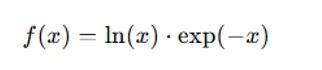
This function exhibits two distinct behaviors:

• The logarithmic component, ln(x), grows very slowly but becomes undefined at x=0x = 0x=0, creating a singularity at the lower limit of integration.
• The exponential component, exp(-x), decays rapidly as xxx increases, especially beyond x=2x.

Such characteristics make it necessary to go beyond simple numerical rules and tailor an approach that respects the behavior of the function across the interval of interest.

Designing a Custom Integration Method

When dealing with special functions, it is helpful to customize your numerical integration approach. Here are a few strategies to consider:

1. Domain Transformation

Transform the interval of integration so that the singularity is either removed or softened. For example, you might map the original interval [0, a] to [0, 1] using a substitution such as x=at, or for more complex behavior, use transformations like x=t2 or x=et, depending on the nature of the singularity.

2. Adaptive Quadrature

Adaptive quadrature techniques adjust the step size based on the behavior of the function. Where the function changes rapidly, the method takes smaller steps, increasing accuracy. MATLAB’s integral() function uses adaptive quadrature internally, but you can implement your own version using recursive subdivision.

3. Weighted Quadrature

Weighted quadrature rules modify the integration formula by applying weights that reflect the expected behavior of the function. For instance, Gaussian quadrature with a logarithmic weight function may yield better results when the integrand contains logarithmic terms.

4. Avoiding the Singularity at x=0x = 0x=0

Since ln(x) is undefined at zero, numerical integration over intervals that start at zero must be handled carefully. One practical approach is to avoid integrating directly at zero by shifting the interval slightly. Instead of integrating from [0, 2], integrate from [ε, 2], where ε is a small positive number like 1e-6. Alternatively, you could estimate the singular contribution analytically and then combine it with numerical results from the rest of the domain.

Implementing the Method in MATLAB

Once the method is designed, implementing it in MATLAB involves defining:

• The function to integrate
• The limits of integration (adjusted if necessary)
• The rule to apply (e.g., midpoint, trapezoidal, Simpson’s)
• Optional: an adaptive mechanism to refine the step size

Start with small intervals and verify the result using a known integration value or a MATLAB built-in method like integral or quadgk.

Comparison with Standard Methods

After computing the integral using your custom method, it is good practice to compare your results with standard methods. MATLAB provides several built-in tools such as:

• trapz for the trapezoidal rule
• integral for adaptive quadrature
• quadgk for Gauss-Kronrod quadrature

By running all methods and comparing:

• Computed integral values
• Computational time
• Number of function evaluations

you can evaluate the accuracy and efficiency of your custom method. Plotting the error versus the number of intervals can also help you understand convergence behavior.

Part 2: Solving Differential Equations Using Iterative Numerical Integration

Another type of assignment that students frequently encounter involves solving differential equations numerically. While MATLAB has powerful built-in solvers like ode45, students are often required to implement their own solvers using basic numerical methods. A common approach is to reformulate the differential equation into an integral equation and then solve it iteratively using a numerical integration rule such as Simpson’s Rule.

Reformulating the Differential Equation

Take a nonlinear first-order ODE like:

This transformation turns the differential equation into an integral equation, where the unknown function appears inside the integral. This makes the problem well-suited for an iterative solution.

Discretizing the Domain

Divide the interval [0, 2] into small subintervals of equal length

• Let h be the step size
• Define an array x = 0:h:2 to represent the grid points
• Initialize y(1) = y0 = 1

The goal is to compute the value of y(i) for each x(i) using numerical integration over the interval [0, x(i)].

Applying Simpson’s Rule Iteratively

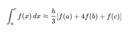
Simpson’s Rule estimates the integral of a function over an interval by fitting a quadratic polynomial through three points. For evenly spaced nodes a, b, and c, Simpson’s Rule gives:

To apply this iteratively:

• At each x(i), compute the integral from 0 to x(i)
• Approximate f(s) = s * exp(-y(s)) at each previous point
• Use the known values of y up to x(i) to compute the integral
• Update y(i) = y(0) + integral_result

This process is repeated until all values of y(x) are computed across the domain.

MATLAB Implementation Tips

• Preallocate arrays for performance
• Use a for-loop to iterate through each x-value
• Store intermediate values of y to use in the next step’s integration
• Plot the final result using plot(x, y) to visualize the solution

Analyzing Error and Stability

Solving nonlinear ODEs numerically can introduce both truncation and round-off errors. As you approach the upper bound of the interval (e.g., x = 2), small errors may be amplified, especially in nonlinear equations.

To address this:

• Use a small step size (e.g., h = 0.01)
• Compare results with a finer grid (smaller h) to assess convergence
• Monitor the difference between successive iterations

If large oscillations or divergence occur, consider using a predictor-corrector method or increasing numerical precision using MATLAB’s vpa() from the Symbolic Math Toolbox.

Conclusion

Assignments involving numerical integration and differential equations often serve as a bridge between theoretical mathematics and practical computation. In tackling such problems, students are expected to understand not only the math but also the logic behind designing computational strategies and implementing them efficiently in MATLAB. When faced with a function that contains singularities or complex behaviors, standard numerical methods may fall short. In such cases, designing a custom integration rule by understanding the function's behavior, applying transformations, and implementing adaptive or weighted techniques can lead to more accurate results. These strategies help students gain a deeper appreciation of numerical analysis, especially when compared with built-in tools like Simpson’s Rule or Gaussian Quadrature. Similarly, differential equations that resist analytical solutions can often be approached through iterative numerical methods. Reformulating them into integral equations provides a pathway to solve them using rules like Simpson’s. While MATLAB offers built-in ODE solvers, implementing your own numerical method enhances conceptual understanding and allows for deeper exploration into error behavior, convergence, and computational stability. Overall, mastering these techniques enables students to solve their numerical integration assignment with confidence. The ability to build custom solutions in MATLAB, analyze errors, and interpret results is a valuable skill that goes beyond the classroom. Whether you’re working on a homework task or a real-world application, approaching problems systematically with a focus on both theory and implementation is the key to success in numerical computing.