How to Solve MATLAB Assignments on Control Systems and System Performance

Dr. Samuel Carter

United States

Control Systems

Dr. Samuel Carter, with over 10 years of experience in control systems and system performance, holds a Ph.D. in Electrical Engineering from the University of Aberdeen, UK.

Hire Me To Do Your Control Systems Assignment

1. Understanding First-Order Systems

First-order systems are the simplest type of dynamic systems, yet they are incredibly important. They are characterized by a single energy storage element—such as a capacitor in an RC circuit or an inductor in an RL circuit—and can be described by a single differential equation. A typical first-order system has a transfer function of the form:

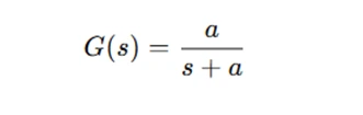
where:

• a is a constant that determines the system’s time constant,
• s is the complex frequency variable in the Laplace domain.

Mathematical Analysis of First-Order Systems

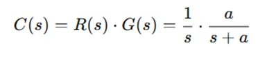
For a given first-order system, you often start by finding its response to a unit step input. The transfer function for the system in the Laplace domain is given by:

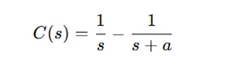
Performing a partial fraction expansion on this expression allows you to rewrite it in a form that is easier to invert back to the time domain. The expansion typically yields:

Taking the inverse Laplace transform, you obtain the time response:

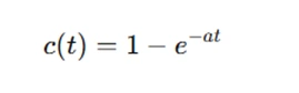
Here, the parameter a is key. It determines the time constant τ of the system, where:

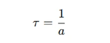
The time constant is a measure of how quickly the system responds to a change in input. When t=τ, the system output reaches approximately 63% of its final value.

MATLAB Implementation for First-Order Systems

In MATLAB, you can simulate the step response of a first-order system using the following steps:

• Define the Transfer Function:

Use the tf function to define the transfer function:

a = 5; % Example value for 'a' sys = tf(a, [1 a]);
• Simulate the Step Response:

Use the step command to generate and plot the step response:

step(sys); title('Step Response of a First-Order System'); xlabel('Time (seconds)'); ylabel('Response');
• Analyze the Response:

MATLAB also provides functions such as damp to calculate system parameters, which can help you verify that the time constant τ is indeed 1a

By understanding the theory behind first-order systems and practicing these MATLAB commands, you can quickly analyze and interpret the dynamic behavior of many simple control systems.

2. Analyzing Transient Response Characteristics

A crucial part of studying control systems is analyzing the transient response—the system's reaction from its initial state to its steady-state value. For first-order systems, there are three key performance metrics:

• Time Constant (τ)

As mentioned earlier, the time constant τ=1/a determines how quickly the system responds. It is the time required for the system to reach 63% of its final value after a step input.

• Rise Time (Tr)

The rise time is defined as the time it takes for the system's response to increase from 10% to 90% of its final value. For a first-order system, the rise time can be determined by evaluating the exponential response at 10% and 90% levels, and then calculating the time difference between these two points.

• Settling Time (Ts)

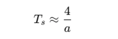
The settling time is the duration required for the system's response to remain within a specific percentage (commonly 2%) of its final value. For many first-order systems, an approximate formula is:



Using MATLAB, you can extract these performance characteristics by examining the step response plot and using built-in functions to measure these time metrics.

3. Exploring Second-Order Systems

Second-order systems are more complex than first-order systems and are represented by a second-order differential equation. The standard form of a second-order system's transfer function is:

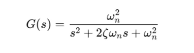
Here:

• ωn is the natural frequency,
• ζ (zeta) is the damping ratio.

Damping and Its Effects

The damping ratio ζ (zeta) critically influences the system's response:

• Underdamped (0<ζ<1): The system exhibits oscillatory behavior with a decaying amplitude.
• Critically Damped (ζ=1): The system reaches steady state as quickly as possible without oscillations.
• Overdamped (ζ>1): The system returns to steady state slowly, with no oscillations.
• Undamped (ζ=0): The system oscillates indefinitely, which is rare in practical applications due to the absence of energy dissipation.

Key Performance Metrics for Second-Order Systems

In addition to the metrics discussed for first-order systems, second-order systems introduce several new performance measures:

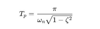
Peak Time (Tp)

Peak time is the time taken for the system to reach its first maximum overshoot following a step input. For an underdamped system, it is given by:

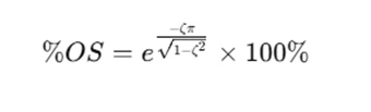
Maximum Overshoot (%OS)

The maximum overshoot quantifies how much the peak level exceeds the steady-state value. It is typically expressed as a percentage and can be calculated as:

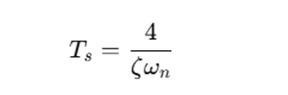
Settling Time (Ts)

For a second-order system, the settling time is approximated by:

MATLAB Implementation for Second-Order Systems

To simulate a second-order system in MATLAB, follow these steps:

• Define the System Parameters:

Suppose you have a system where ωn=4 rad/s and ζ=0.375. You can define the transfer function as:

omega_n = 4; zeta = 0.375; num = omega_n^2; den = [1 2*zeta*omega_n omega_n^2]; sys2 = tf(num, den);
• Plot the Step Response:

Simulate and analyze the response:

step(sys2); title('Step Response of a Second-Order System'); xlabel('Time (seconds)'); ylabel('Response'); grid on;
• Analyze Performance Metrics:

Use MATLAB functions like stepinfo to extract key performance data:

info = stepinfo(sys2); disp(info);

This will provide you with information on the rise time, peak time, overshoot, and settling time, allowing you to compare theoretical predictions with simulation results.

4. Simulating and Analyzing Control Systems in MATLAB

MATLAB offers a robust environment for simulating and analyzing both first-order and second-order systems. Here are some general tips and best practices:

Setting Up Your MATLAB Environment

Before diving into your assignment, make sure you have the Control System Toolbox installed. This toolbox includes all the functions you need for modeling, analyzing, and designing control systems.

Writing Clear and Modular Code

Break your assignment into smaller, manageable parts:

• Define Parameters: Clearly define all constants and parameters at the beginning of your script.
• Create Transfer Functions: Use the tf command to create models for your systems.
• Simulate Responses: Use commands such as step, impulse, or lsim to simulate different types of inputs.
• Analyze Results: Store your simulation data and use MATLAB’s plotting functions to visualize the responses. Include proper titles, labels, and legends in your plots to make them easy to interpret.

Verifying Your Results

Always compare your MATLAB simulation results with theoretical predictions. For example:

• For a first-order system, verify that the time constant τ computed in MATLAB matches 1a.
• For a second-order system, check that the computed damping ratio and natural frequency from the simulation align with your theoretical calculations.

By verifying your results, you ensure that your model is correct and that you fully understand the system’s dynamics.

5. Practical Examples and Exercises

Let’s look at a couple of examples that illustrate how you can apply these concepts in your MATLAB assignments.

Example 1: First-Order System Simulation

Suppose you are given a first-order system with the transfer function:

Steps to Analyze:

• Define the system in MATLAB:
a = 5; sys = tf(a, [1 a]);
• Plot the Step Response:
step(sys); title('Step Response of a First-Order System with a = 5'); xlabel('Time (seconds)'); ylabel('Response'); grid on;
• Extract Performance Data: Use the stepinfo function to get details such as rise time and settling time:
info = stepinfo(sys); disp(info);

Compare the time constant τ=1/5 with the data provided by stepinfo

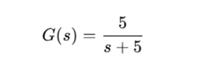
Example 2: Second-Order System Simulation

Consider a second-order system characterized by:

Analysis:

• Determine System Parameters:

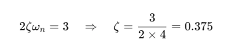
The natural frequency ωn is given by 16=4 rad/s.

The damping ratio ζ is calculated using the coefficient of s:



• Define the System in MATLAB:
omega_n = 4; zeta = 0.375; num = omega_n^2; den = [1 2*zeta*omega_n omega_n^2]; sys2 = tf(num, den);
• Simulate the Step Response:
step(sys2); title('Step Response of a Second-Order System'); xlabel('Time (seconds)'); ylabel('Response'); grid on;
• Analyze Key Metrics: Extract rise time, peak time, maximum overshoot, and settling time using:
info2 = stepinfo(sys2); disp(info2);

This example not only reinforces the theoretical concepts but also demonstrates how MATLAB can be used to validate your calculations.

Conclusion

Understanding and simulating control systems using MATLAB can be challenging at first, but with a structured approach and consistent practice, you can master the concepts of first-order and second-order systems. By following the steps outlined in this guide—from analyzing the basic transfer functions and transient responses to simulating system behaviors in MATLAB—you will build the confidence and skills needed to tackle any MATLAB assignment related to control systems.

Remember, the key to success lies in breaking down the problem, leveraging MATLAB’s powerful tools, and verifying your theoretical predictions with simulation results. Whether you’re working on a simple RC circuit or a more complex mass-spring-damper system, the principles remain the same.