How to Tackle Complex MATLAB Capstone Project Using Multigrid Method

Capstone projects are a significant part of many academic programs, providing an opportunity to demonstrate your knowledge and skills. If you’re working on a MATLAB-based capstone, such as solving complex mathematical problems with the multigrid method applied to the heat equation, it’s essential to understand the process. These types of projects not only test your ability to grasp advanced numerical methods but also challenge you to implement them effectively using programming languages like MATLAB.
In this blog post, we’ll explore the steps to help you to solve your Matlab assignment, whether you’re working on a multigrid method for the heat equation or any other similar computational problem. We’ll focus on breaking down the assignment into manageable tasks, guiding you through the coding process, and offering tips to refine your project.

Step 1: Understand the Problem
The first and most important step in any capstone project is to fully understand the problem you are solving. For a MATLAB project like the Multigrid Method Applied to the Heat Equation, it’s crucial to break down the problem into its core components and understand the mathematical concepts that underpin it.
Multigrid Method:
The multigrid method is a powerful algorithm for solving large linear systems of equations, often arising from discretized partial differential equations (PDEs) like the heat equation. It works by solving the equation at multiple levels of resolution, which improves computational efficiency. Multigrid methods typically involve:
- Smoothing: Reducing high-frequency errors on the fine grid.
- Coarse Grid Correction: Moving to coarser grids to correct low-frequency errors, then refining back to the finer grids.
- Iterative Refinement: Repeating the smoothing and coarse grid correction steps until the solution converges.
Heat Equation:
The heat equation is a PDE that models the distribution of heat in a given region over time. It is written as:
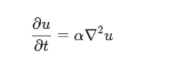
Where:
- u represents the temperature at a point in space and time.
- α is the thermal diffusivity, a constant that dictates how fast heat spreads through a medium.
- ∇2 is the Laplacian operator, representing the spatial derivatives of temperature.
Understanding both the theory of the multigrid method and the specific problem you are solving will provide a solid foundation for your MATLAB implementation. Be sure to read through any suggested textbooks, such as A Multigrid Tutorial by Briggs, to grasp the fundamental principles behind these techniques.
Step 2: Break Down the Assignment
Once you understand the problem, it’s time to break it down into smaller, manageable components. MATLAB assignments often involve multiple stages, including grid creation, discretization, and solving the problem using specific methods like multigrid.
Define the Problem:
Before you write any code, define the variables and parameters you’ll be working with. For the heat equation, this typically involves the spatial domain, time steps, and the initial temperature distribution.
Here are some initial parameters you might set up in your MATLAB code:
Nx = 100; % Number of grid points in space
Nt = 500; % Number of time steps
L = 1; % Length of the domain
T = 0.5; % Final time
dx = L/(Nx-1); % Spatial step size
dt = T/Nt; % Time step size
Discretize the Equation:
For the heat equation, discretization involves approximating the continuous variables in both space and time. Typically, you’ll use finite difference methods to discretize the spatial and temporal derivatives. For instance:
- Spatial discretization: You can use a grid of points where each point represents the temperature at a specific location in space. The Laplacian operator is approximated using finite difference formulas.
- Time discretization: Similarly, the time derivative is approximated using methods like the forward Euler method or the backward Euler method.
In the case of the heat equation, after discretization, you will end up with a system of equations that you can solve using iterative methods such as the multigrid method.
Implement the Multigrid Method:
The multigrid method involves multiple grid levels with different resolutions. You start by solving the problem on a fine grid, then gradually move to coarser grids to eliminate low-frequency errors, before refining back to the fine grid. Here are the core components of the method:
- Smoothing: Apply a simple iterative method (e.g., Gauss-Seidel) to smooth the solution and reduce high-frequency errors.
- Coarse Grid Correction: Use the solution from the coarse grid to correct the finer grid’s solution.
- Interpolation and Restriction: Interpolate the solution from the coarse grid back to the fine grid and restrict the solution from the fine grid to the coarse grid.
Step 3: Write the MATLAB Code
Now that you’ve broken the assignment into manageable tasks, it’s time to start writing the MATLAB code. This will involve setting up your grid, initializing your variables, and implementing the multigrid method. Below is a simple framework to help you get started.
Set Up the Grid:
You’ll first need to create a grid of points for both space and time. Here’s how you can set that up:
Nx = 100; % Number of grid points in space
Nt = 500; % Number of time steps
L = 1; % Length of the domain
T = 0.5; % Final time
dx = L/(Nx-1); % Spatial step size
dt = T/Nt; % Time step siz
Initialize the Solution:
Next, you’ll initialize the temperature distribution. You may have a specific initial condition depending on your problem, but here’s a generic setup:
u = zeros(Nx, Nt); % Initialize the temperature field
u(:,1) = initial_conditions(); % Set the initial temperature distribution
Implement the Multigrid Method:
The multigrid method requires functions for smoothing, restriction, and interpolation. Let’s start by implementing a simple smoothing function:
function u_smooth = smooth(u, Nx, Nt)
    % Apply Gauss-Seidel relaxation
    for i = 2:Nx-1
        for j = 2:Nt-1
            u(i,j) = 0.5 * (u(i+1,j) + u(i-1,j) + u(i,j+1) + u(i,j-1));
        end
    end
    u_smooth = u;
end
Time Stepping:
Use a loop to implement the time-stepping procedure and update the solution at each step. Each iteration will involve smoothing and applying the multigrid method:
for t = 1:Nt-1
    % Perform smoothing and multigrid steps
    u = smooth(u, Nx, Nt);
    % Apply other multigrid components here (restriction, coarse grid correction)
End
Visualize the Solution:
Finally, it’s always important to visualize your results. MATLAB offers several plotting functions that you can use to display your solution. A surface plot of the temperature distribution might look like this:
surf(u);
title('Heat Distribution');
xlabel('Space');
ylabel('Time');
zlabel('Temperature');
Step 4: Test and Debug
Once you’ve written your code, it’s essential to test it and debug any issues that arise. It’s a good idea to start with simple test cases to ensure that the basic components of your program are working. For example, you could test your code with smaller grids and fewer time steps to quickly identify any errors.
Refining the Solution:
Once your initial tests pass, refine your code by adjusting the grid size, time steps, and solver parameters. Keep in mind that numerical methods are sensitive to these parameters, so small adjustments can significantly improve accuracy or performance.
Step 5: Document the Code and Results
As this is a capstone project, your instructor will likely expect clear documentation. This includes:
- Comments: Write comments throughout your code to explain the functionality of each section.
- Results: Include the numerical results and any relevant plots or data that demonstrate the effectiveness of your solution.
Conclusion
Tackling a MATLAB-based capstone project, like applying the multigrid method to the heat equation, may seem overwhelming at first, but by breaking the problem down into smaller, manageable components, you can approach it with confidence. Understanding the mathematical theory behind the method, carefully discretizing the equations, and implementing the solution step by step are crucial to success. The multigrid method, with its efficiency and power in solving large linear systems, can be a complex algorithm to implement, but with a structured approach, it becomes an achievable task.
Remember to test your code thoroughly, refine your implementation, and document your results clearly. As you work through your project, you’ll not only demonstrate your understanding of numerical methods but also improve your coding skills in MATLAB, which will be valuable in future assignments and professional work. Keep in mind that a well-documented, well-tested project, combined with a clear explanation of your results, will set you up for success in completing your capstone and in showcasing your problem-solving abilities.
By following these steps and staying focused on your goal, you’ll be able to produce a comprehensive, effective solution that showcases both your technical knowledge and programming skills. With dedication and careful planning, you can confidently complete your MATLAB capstone project and make a meaningful contribution to your academic field.