How to Address MATLAB Assignments on Fourier Transforms and EEG Signal Analysis

MATLAB assignments, especially those involving Fourier Transforms and EEG signal analysis, can initially seem complex due to the wide range of concepts and techniques involved. Whether you’re working with continuous and discrete Fourier transforms (DFT and FFT) or diving into practical applications like EEG signal processing, understanding the underlying principles and systematic approaches will help you excel in these types of assignments. This guide provides step-by-step instructions on how to solve your signal processing assignment, offering practical tips, and helping you navigate through MATLAB functions, analysis techniques, and more. By following this approach, you will not only complete your Fourier Transform assignment but also build a deeper understanding of signal processing concepts.
Understanding Fourier Transforms and Signal Processing
Fourier Transforms are essential tools for analyzing signals in the frequency domain, and they play a significant role in MATLAB assignments related to signal processing. Before diving into solving a specific problem, let’s first understand the key concepts around continuous and discrete Fourier transforms.

Continuous Fourier Transform (CFT)
The Continuous Fourier Transform (CFT) is a mathematical operation that converts a time-domain signal into its frequency-domain counterpart. In practical terms, this means that CFT can show how much of each frequency is present in a signal at a given time. This transformation is fundamental when dealing with real-world signals like audio, communications, and EEG data. The CFT produces a continuous representation of the signal’s frequency spectrum, which may have infinite values, making it important to handle these appropriately during the plotting process.
When you’re tasked with plotting the CFT, you’ll often need to represent infinite values with an upward-pointing arrow. In MATLAB, you can use the stem() function with "^" markers to denote these infinite values. To handle this, MATLAB functions like find(), subs(), or isinf() can be helpful in locating and marking these infinite points.
Discrete Fourier Transform (DFT)
The Discrete Fourier Transform (DFT) is the sampled counterpart of the CFT. In MATLAB, the DFT is computed using the Fast Fourier Transform (FFT) algorithm, which efficiently calculates the DFT of discrete signals. Unlike the CFT, the DFT is inherently periodic and provides a discrete representation of the frequency spectrum.
The DFT allows for a more practical analysis of real-world signals, which are sampled at discrete time intervals. When plotting DFT results in MATLAB, you need to apply functions like fftshift() to shift the zero frequency component to the center of the plot, making it easier to visualize the frequency spectrum. Additionally, it’s essential to ensure that your frequency axes and units are correctly labeled to avoid confusion.
Step-by-Step Guide for Solving Fourier Transform Assignments
Fourier transforms can seem daunting at first, but with a systematic approach, solving assignments involving these concepts becomes much more manageable. In this section, we'll break down the key steps to follow when working on a Fourier Transform assignment, focusing on understanding the signal, performing the necessary calculations, and visualizing the results effectively. By following this step-by-step guide, you’ll gain practical experience working with Fourier Transforms in MATLAB, which is an essential skill for signal processing tasks. Whether you are dealing with continuous or discrete Fourier transforms, this guide will help you handle these problems with confidence.
1. Start by Understanding the Signal
The first step to solve your matlab assignment related to Fourier transforms is understanding the signal you’re working with. In the example provided, the signal is a combination of an exponential term and a cosine term:
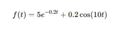
The signal is sampled at a rate of 5 kHz, and you’re tasked with plotting both the continuous Fourier transform (CFT) and discrete Fourier transform (DFT) for various sampling periods (like 10, 50, and 100 seconds).
To start, you need to plot the time-domain signal, f(t), over a specified time range (e.g., 10 seconds). This will give you an initial visual of the signal’s behavior. You can use the MATLAB plot() function to create this plot and analyze the shape and components of the signal.
2. Generate the Continuous Fourier Transform (CFT)
Once you’ve plotted the time-domain signal, the next step is to compute its continuous Fourier transform. This process involves converting the signal from the time domain to the frequency domain, which can be done using the analytical form of the Fourier transform for the given signal. In MATLAB, you may use symbolic math functions to derive the CFT of the signal.
When plotting the CFT, remember that the amplitude of the frequency components may approach infinity at certain frequencies. In these cases, you can use the stem() function with "upward arrows" to denote infinite values. The CFT plot will show a continuous representation of the frequency spectrum, and you should make sure that all frequency axes have the same limits for consistency.
3. Generate the Discrete Fourier Transform (DFT)
Next, you’ll compute the Discrete Fourier Transform (DFT) using MATLAB’s fft() function. This step involves sampling the time-domain signal at discrete intervals and converting it to the frequency domain. As mentioned earlier, you’ll need to apply fftshift() to center the frequency spectrum and make the plot easier to interpret.
In the DFT plot, you should expect to see peaks corresponding to the frequencies present in the signal. The peaks will be influenced by the sampling rate, so make sure to create plots for different sampling durations (such as 10, 50, and 100 seconds). These variations will show you how the DFT approximation changes as the sampling period increases.
4. Comparing Continuous and Discrete Fourier Transforms
After plotting both the CFT and DFT for various sampling durations, compare the results. The assignment asks you to analyze whether the DFT corresponds well with the theoretical CFT. In general, the DFT should closely match the CFT, but there will be some differences due to the discrete nature of the DFT.
As you analyze the plots, focus on the two key components:
- Peaks that remain constant in amplitude as the sampling period increases.
- Peaks that change in amplitude with increasing sampling duration.
These observations will help you understand how the time-domain components of the signal, such as the exponential and cosine terms, affect the frequency-domain representation.
5. Understanding Amplitude Relationships
One critical part of this assignment is understanding the relationship between the amplitude of the Fourier transform (or FFT) and the components of the time-domain signal. The assignment asks you to examine how the amplitude of the FFT relates to the exponential and sine wave components of the signal.
To explore this, try altering one coefficient at a time in the signal and observing the changes in the frequency spectrum. By doing this, you can see how each part of the signal contributes to the overall Fourier transform.
Practical Application: EEG Signal Processing
In the second part of the assignment, you’ll be tasked with analyzing an artificial EEG signal. EEG signals are commonly used in neuroscience and clinical practice to monitor brain activity. These signals contain several frequency components, each corresponding to different brain wave types (e.g., alpha, beta, delta, theta). The challenge in this part of the assignment is to analyze the underlying frequencies in the EEG signal and identify various wave types.
1. Load and Pre-process the EEG Data
Begin by loading the EEG signal data (e.g., in MATLAB .mat file format). The signal is sampled at 1 kHz, and you’ll need to analyze the frequency components within this signal. Start by plotting the signal in the time domain to visually inspect it and get a sense of its overall structure.
2. Fourier Transform of the EEG Signal
Once the signal is loaded, the next step is to transform it from the time domain to the frequency domain. Use the fft() function to compute the discrete Fourier transform (DFT) of the signal. You can then apply fftshift() to center the frequency spectrum and make the resulting plot easier to analyze.
3. Identifying EEG Wave Types
EEG signals are typically divided into different frequency bands or wave types. The common wave types and their frequency ranges are:
- Delta waves (0.5-2 Hz)
- Theta waves (4-7 Hz)
- Alpha waves (8-15 Hz)
- Beta waves (16-31 Hz)
- Gamma waves (32-100 Hz)
By analyzing the frequency spectrum of the EEG signal, you can identify the presence of these wave types. Look for peaks in the spectrum that fall within these frequency ranges and interpret them accordingly.
4. Analyzing Dream States
A specific application of EEG signal analysis involves detecting dream states, which are typically characterized by higher-frequency, lower-amplitude signals. In the assignment, you are asked to identify periods where the signal exceeds 75 Hz, as these correspond to when the patient is dreaming. Once you’ve identified these periods, record the duration, frequency, and wave type for each dream state.
5. Noise Analysis in EEG
EEG signals are often contaminated by noise, which can manifest as random or periodic spikes in the frequency spectrum. When analyzing EEG data, it’s important to identify any noise and determine whether it interferes with the underlying brain wave patterns. If noise is present, try to determine its frequency and time-domain characteristics. In some cases, noise removal techniques like filtering can help eliminate unwanted components from the signal.
Final Thoughts
Signal processing assignments involving Fourier Transforms and EEG analysis can be challenging, but with a structured approach, you can break them down into manageable steps. By following the steps outlined in this guide, you’ll be able to understand the theory behind Fourier transforms, apply them to real-world signals, and analyze complex data like EEG signals.
As you work through these assignments, keep practicing MATLAB functions such as fft(), fftshift(), plot(), and stem(). These tools will help you visualize and interpret your results effectively. Whether you're analyzing the frequency spectrum of a simple signal or tackling more complex applications like EEG analysis, a systematic approach will allow you to solve these problems efficiently.