Effective Ways to Solve MATLAB Assignment Problems using Fluid Mechanics and Dynamics

MATLAB is a powerful tool that is widely used by students in fields such as engineering, physics, mathematics, and computer science for solving complex problems. Many of these assignments require the combination of analytical methods, numerical techniques, and simulation. This blog will guide students through the process to solve your MATLAB assignment, specifically focusing on problems like mass-spring systems, fluid dynamics, and systems of differential equations. The steps provided below can be adapted for various assignments involving similar concepts.
Step 1: Understanding the Problem
The first and most important step in solving any assignment is to thoroughly understand the problem. Before diving into MATLAB or even doing hand calculations, it's crucial to comprehend the system being described in the problem statement.
Breaking Down the Problem

Carefully read through the assignment question and identify the key components. Are you dealing with a dynamic system like a mass-spring system, or are you solving a fluid flow or mixing problem? Each system has different characteristics and mathematical models.
For example, in a fluid dynamics problem involving interconnected tanks, the objective is usually to determine the concentration or mass of a substance (e.g., salt) in each tank over time. The problem would typically provide information about the flow rates between tanks and the concentration of the substance in the inflow, as well as the initial conditions of the system.
In a spring-mass system, you would need to identify forces acting on the mass, such as restoring forces (spring force) and damping forces. These problems often involve differential equations describing how the position of the mass changes over time.
Identifying Key Variables and Parameters
After understanding the problem, identify all the variables and parameters involved in the system. For example, in a mass-spring system, these might include:
- Mass (m): The mass attached to the spring.
- Spring constant (k): The stiffness of the spring.
- Damping coefficient (b): The amount of resistance to motion due to damping.
- Displacement (x(t)): The position of the mass as a function of time.
In a mixing problem, the variables might include:
- Volume of the tanks: The size of each tank.
- Flow rates: The rates at which liquid flows between tanks or into/out of the tanks.
- Concentration of the substance: The amount of the substance (e.g., salt) per unit volume of liquid.
Defining the Objective
Finally, determine the objective of the problem. Are you tasked with finding the mass of salt in a tank at a given time, the displacement of a mass in a spring-mass system, or the solution to a system of coupled differential equations? This will guide your approach to solving the problem.
Step 2: Formulating the Mathematical Model
Once you have a good understanding of the problem, the next step is to translate it into a mathematical model. This is where you express the problem in terms of equations, typically differential equations, that describe the behavior of the system.
Defining the Governing Equations
For most engineering problems, you will encounter ordinary differential equations (ODEs). These equations are used to describe systems that change over time. The form of the ODE depends on the type of system you are dealing with.
For a mixing problem involving interconnected tanks: You would write mass balance equations for each tank. For example, if Tank A has a flow rate of 3 L/min into Tank B, a flow rate of 1 L/min out of Tank B, and an inflow of a brine solution with a known concentration, the rate of change of mass in Tank A can be written as:
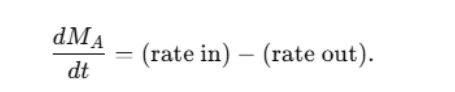
Here, MA is the mass of the substance in Tank A, and similar equations can be written for Tank B.
For a spring-mass system: The governing equation can be derived from Newton’s second law:
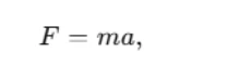
where F is the total force acting on the mass, m is the mass, and aaa is the acceleration of the mass. For a spring-mass system with damping, the force includes the spring force and damping force:
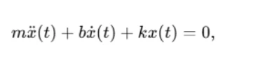
where:
- m is the mass,
- b is the damping coefficient,
- k is the spring constant, and
- x(t) is the displacement of the mass at time t.
For more complex systems, such as systems with multiple coupled masses and springs, you would need to write a system of differential equations, one for each mass.
Initial and Boundary Conditions
Next, define the initial and boundary conditions for the system. These are the known values at the start of the problem (e.g., initial displacement or velocity of a mass). For a spring-mass system, the initial conditions could look like:
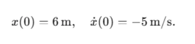
These conditions will be used to solve the differential equations numerically and analytically.
Step 3: Solving the Problem Analytically (Hand Calculations)
In many assignments, you are expected to solve the differential equations analytically. This means finding a solution using traditional mathematical techniques, such as separation of variables, integrating factors, or Laplace transforms.
Analytical Methods for Simple ODEs
For simple first-order linear differential equations, you might be able to find an analytical solution using techniques like separation of variables or integrating factors. For example, if you have an equation like:
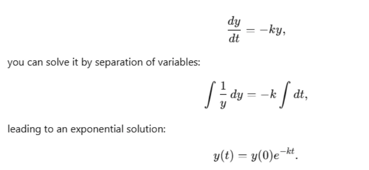
Analytical Solutions for Spring-Mass Systems
For a spring-mass system, the solution depends on the damping conditions. If the system is underdamped, you can find the displacement as a sinusoidal function, while for overdamped or critically damped systems, the solution involves exponential decay terms. Solving these equations analytically typically involves using the characteristic equation derived from the homogeneous differential equation.
Step 4: Solving the Problem Numerically Using MATLAB
For most real-world problems, especially when dealing with complex systems or systems without simple analytical solutions, numerical methods are used. MATLAB provides a variety of functions to solve ODEs numerically, with ode45 being one of the most commonly used functions.
Using ode45 to Solve ODEs
The ode45 function in MATLAB uses the Runge-Kutta method to numerically solve first-order differential equations. To use ode45, you need to define the system of equations in a function handle format and specify initial conditions.
For example, for a spring-mass system:
% Define the ODE
ode = @(t, y) [y(2); -k/m*y(1) - b/m*y(2)];

% Initial conditions
y0 = [6; -5];  % Initial displacement and velocity

% Time span
tspan = [0 10];  % Solve from t=0 to t=10

% Solve the ODE
[t, y] = ode45(ode, tspan, y0);

% Plot the results
figure;
plot(t, y(:, 1), 'b', 'LineWidth', 2);
xlabel('Time (s)');
ylabel('Displacement (m)');
title('Displacement vs Time for Spring-Mass System');
grid on;
In this example, ode45 solves the second-order ODE by converting it into a system of first-order equations and then numerically integrates it over the specified time span.
Solving Systems of Equations
If you have multiple coupled equations, such as in the case of interconnected tanks or multiple masses and springs, you can represent the system as a set of first-order equations and solve them using ode45 in a similar manner.
For interconnected tanks, you would have two differential equations, one for each tank, and solve them as a system:
ode = @(t, y) [inflow_A - outflow_A - flow_AB; flow_AB - outflow_B];

% Initial conditions
y0 = [0; 20];  % Initial conditions for the masses of salt

% Solve the system
[t, y] = ode45(ode, tspan, y0);
Step 5: Creating a Simulink Model
Simulink, a graphical extension of MATLAB, is used for modeling and simulating dynamic systems. It provides an intuitive interface where you can design your model using blocks and interconnect them. For many students, Simulink can be a more visual way to understand and simulate systems of equations.
Building a Simulink Model for a Spring-Mass System
To create a Simulink model:
- Open Simulink by typing simulink in the MATLAB command window.
- Drag and drop the relevant blocks, such as Integrator, Sum, Gain, and Scope, to model the system.
- Define the system parameters (mass, damping, spring constant) in the block parameters.
- Connect the blocks to represent the physical system, then run the simulation.
Simulink allows you to model the system graphically and visualize the results in real-time.
Step 6: Plotting and Analyzing the Results
Once you have solved the problem numerically and/or created a Simulink model, it's time to visualize the results. MATLAB provides several plotting functions to help you create clear and informative graphs.
Plotting Solutions
You can plot both the analytical and numerical solutions on the same graph to compare their behavior. For example:
% Analytical solution
x_analytic = exp(-b/(2*m)*t) .* (A*cos(omega*t) + B*sin(omega*t));

% Numerical solution
[t, y] = ode45(@(t, y) [y(2); -k/m*y(1) - b/m*y(2)], tspan, y0);

% Plot both solutions
figure;
hold on;
plot(t, x_analytic, 'r', 'LineWidth', 2);
plot(t, y(:,1), 'b', 'LineWidth', 2);
legend('Analytical', 'Numerical');
xlabel('Time (s)');
ylabel('Displacement (m)');
title('Comparing Analytical and Numerical Solutions');
grid on;
hold off;
Refining the Plots
Ensure your plots are well-formatted. Use appropriate axis labels, titles, legends, and grid lines. MATLAB allows customization of line colors, styles, and markers to make your graphs more readable and professional.
Conclusion
Solving MATLAB assignments involves a systematic approach, beginning with understanding the problem, formulating the appropriate mathematical model, solving it both analytically and numerically, and simulating the system using tools like Simulink. By following these steps and using the right functions in MATLAB, you can efficiently solve complex problems and gain a deeper understanding of the underlying physical principles.