How to Successfully Handle MATLAB Assignments in Aerodynamics

MATLAB assignments, especially those related to aerodynamics, can seem daunting at first. However, with a structured approach, you can tackle aerodynamics assignment effectively. This blog will help you understand the general steps to solve MATLAB assignments related to aerodynamics, such as the one described above. The focus will be on key concepts, strategies, and MATLAB functions that are commonly used in these types of assignments.
Understanding the Assignment
The first step in solving any MATLAB assignment is to thoroughly understand the problem statement. In the example provided, the goal is to compute the pressure distribution about a symmetric airfoil using a series of sources and sinks. Here's a breakdown of the key tasks involved:
- Generalize the velocity distribution for n sources/sinks.
- Transform the coordinates to place the airfoil in the standard position.
- Compute the pressure coefficient (Cp).
- Generate streamlines and solve for source/sink strengths.
- Compute and analyze the RMS error between the predicted and published pressure distribution.
- Document your results and MATLAB code in a report.

Step-by-Step Approach
1. Generalize the Velocity Distribution
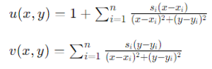
The velocity distribution for a flow over n sources/sinks is given by:
Here, (xi,yi)(x_i, y_i)(xi,yi) are the locations of the sources/sinks and sis_isi are the source/sink strengths. Implementing this in MATLAB involves creating functions that compute these velocities.
MATLAB Implementation:
function [u, v] = velocity_distribution(x, y, x_s, y_s, s)
u = 1;
v = 0;
n = length(s);
for i = 1:n
u = u + s(i) * (x - x_s(i)) / ((x - x_s(i))^2 + (y - y_s(i))^2);
v = v + s(i) * (y - y_s(i)) / ((x - x_s(i))^2 + (y - y_s(i))^2);
end
end
2. Transform the Coordinates
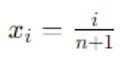
To place the airfoil in the standard position, you need to transform the coordinates such that the leading edge is at x=0x = 0x=0 and the trailing edge at x=1x = 1x=1. This is done by placing the sources/sinks as:
3. Compute the Pressure Coefficient
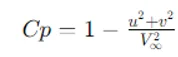
The pressure coefficient is defined as:
MATLAB Implementation:
function Cp = pressure_coefficient(u, v, V_inf)
Cp = 1 - (u.^2 + v.^2) / V_inf^2;
End
4. Generate Streamlines and Solve for Source/Sink Strengths
Using the stream function ψ(x,y)\psi(x, y)ψ(x,y) and ensuring all airfoil points are on the same streamline (i.e., ψ(Xj,Yj)=0\psi(X_j, Y_j) = 0ψ(Xj,Yj)=0), you can solve for the source/sink strengths.
MATLAB Implementation:
% Define airfoil shape points
function [X, Y] = airfoil_shape(t, n)
X = linspace(0, 1, n);
Y = (t/0.20) * (0.2969 * sqrt(X) - 0.1260 * X - 0.3516 * X.^2 + 0.2843 * X.^3 - 0.1015 * X.^4);
end
% Solve for source/sink strengths
function s = solve_source_strengths(X, Y)
n = length(X);
M = zeros(n, n);
R = zeros(n, 1);
for i = 1:n
for j = 1:n
M(i, j) = ... % Define matrix M based on X, Y, and stream function conditions
end
R(i) = 0; % Stream function value should be zero on the airfoil
end
s = M \ R;
end
5. Compute and Analyze the RMS Error
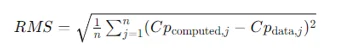
The RMS error helps you compare the predicted and actual pressure distribution:
MATLAB Implementation:
function rms_error = compute_rms_error(Cp_computed, Cp_data)
rms_error = sqrt(mean((Cp_computed - Cp_data).^2));
end
6. Document Your Results
Create a comprehensive report that includes:
- A short introduction
- Plots of the source/sink distribution and pressure coefficients
- Field plots with streamlines, singularity locations, and airfoil points
- RMS error analysis for different numbers of sources
- Your MATLAB code with explanations
Detailed Guide to Solving the Assignment
Let's delve into each step in more detail, focusing on the concepts and practical steps involved.
Generalizing the Velocity Distribution
In aerodynamics, the velocity field around an airfoil can be modeled using a combination of sources and sinks. The goal is to create a mathematical representation that captures the flow characteristics accurately. The equations provided describe the velocity components u(x,y)u(x, y)u(x,y) and v(x,y)v(x, y)v(x,y) in the x and y directions, respectively.
To implement these equations in MATLAB, you need to create a function that computes the velocity at any point (x, y) given the positions and strengths of the sources and sinks. The function iterates through each source/sink, adding their contributions to the overall velocity field.
MATLAB Code Example:
function [u, v] = velocity_distribution(x, y, x_s, y_s, s)
u = 1;
v = 0;
n = length(s);
for i = 1:n
u = u + s(i) * (x - x_s(i)) / ((x - x_s(i))^2 + (y - y_s(i))^2);
v = v + s(i) * (y - y_s(i)) / ((x - x_s(i))^2 + (y - y_s(i))^2);
end
end
This function initializes the velocity components uuu and vvv, then iteratively updates them based on the contributions from each source/sink.
Transforming the Coordinates
To align the airfoil in the standard position, the sources and sinks need to be placed at specific x-coordinates, defined by xi=in+1x_i = \frac{i}{n + 1}xi=n+1i. This transformation ensures that the leading edge of the airfoil is at x=0x = 0x=0 and the trailing edge is at x=1x = 1x=1.
Computing the Pressure Coefficient
The pressure coefficient CpCpCp is a crucial parameter in aerodynamics, representing the pressure distribution over the airfoil. It is computed using the local velocity components uuu and vvv:
Cp=1−u2+v2V∞2Cp = 1 - \frac{u^2 + v^2}{V_\infty^2}Cp=1−V∞2u2+v2
This equation indicates that CpCpCp is inversely related to the square of the local velocity magnitude. In MATLAB, you can create a function to compute CpCpCp at each point on the airfoil.
MATLAB Code Example:
function Cp = pressure_coefficient(u, v, V_inf)
Cp = 1 - (u.^2 + v.^2) / V_inf^2;
End
Generating Streamlines and Solving for Source/Sink Strengths
Streamlines represent the paths followed by fluid particles in the flow field. In MATLAB, you can use the stream function ψ(x,y)\psi(x, y)ψ(x,y) to generate streamlines. The stream function is related to the velocity components by:
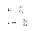
To ensure that all airfoil points lie on the same streamline, you set ψ(Xj,Yj)=0\psi(X_j, Y_j) = 0ψ(Xj,Yj)=0. This creates a system of equations that can be solved for the source/sink strengths sis_isi.
MATLAB Code Example:
% Define airfoil shape points
function [X, Y] = airfoil_shape(t, n)
X = linspace(0, 1, n);
Y = (t/0.20) * (0.2969 * sqrt(X) - 0.1260 * X - 0.3516 * X.^2 + 0.2843 * X.^3 - 0.1015 * X.^4);
end
% Solve for source/sink strengths
function s = solve_source_strengths(X, Y)
n = length(X);
M = zeros(n, n);
R = zeros(n, 1);
for i = 1:n
for j = 1:n
M(i, j) = ... % Define matrix M based on X, Y, and stream function conditions
end
R(i) = 0; % Stream function value should be zero on the airfoil
end
s = M \ R;
end
In the solve_source_strengths function, you construct the matrix MMM and the vector RRR to solve for sss.
Computing and Analyzing the RMS Error
The Root Mean Square (RMS) error measures the difference between the computed pressure coefficients and the actual data. This helps evaluate the accuracy of your model.
MATLAB Code Example:
function rms_error = compute_rms_error(Cp_computed, Cp_data)
rms_error = sqrt(mean((Cp_computed - Cp_data).^2));
end
This function takes the computed and actual CpCpCp values and calculates the RMS error, providing a quantitative measure of the model's accuracy.
Documenting Your Results
A well-documented report is essential for presenting your findings clearly. Your report should include:
- Introduction: Briefly describe the problem and objectives.
- Source/Sink Distribution: Plot and analyze the distribution of sources/sinks.
- Pressure Coefficient: Compare the predicted and actual CpCpCp values.
- Field Plots: Include streamlines, singularity locations, and airfoil points.
- RMS Error Analysis: Present the RMS error for different numbers of sources.
- MATLAB Code: Provide your code with explanations.
Tips for Success
- Understand the Theory: Before diving into MATLAB, make sure you understand the aerodynamic theory and mathematical equations involved.
- Break Down the Problem: Divide the assignment into smaller tasks and tackle them one by one.
- Validate Your Results: Continuously check your results against known solutions or data to ensure accuracy.
- Use Built-In Functions: MATLAB has powerful built-in functions like interp1 for interpolation and ode45 for solving differential equations. Utilize them to simplify your code.
- Document Your Code: Comment your MATLAB code extensively to explain what each part does.
Conclusion
Solving MATLAB assignments in aerodynamics involves a combination of theoretical knowledge and practical programming skills. By following a structured approach and leveraging MATLAB's capabilities, you can efficiently tackle assignments like computing the pressure distribution around an airfoil. Remember, practice and continuous learning are key to solving these assignments effectively.