How to Solve MATLAB Assignment on 2D Heat Equation Using Multigrid Method

Numerical simulations are central to understanding physical systems in engineering and science. One of the most studied partial differential equations in this domain is the heat equation, especially in two spatial dimensions. The 2D heat equation describes how temperature evolves within a surface or volume over time and is widely used in thermal engineering, fluid mechanics, and computational physics. MATLAB, due to its intuitive syntax and strong matrix capabilities, is often the preferred tool for students working on such simulations. However, students frequently struggle with optimizing their codes, especially when dealing with complex systems that include non-uniform heat sources, non-zero boundary conditions, and scalability challenges. This is where the Multigrid method becomes essential.
In this blog, we will walk through a general, conceptual, and practical guide to solving the 2D heat equation over time using the Multigrid method. This guide aims to provide clarity for students who are either learning this topic for the first time or those who are stuck trying to solve their MATLAB assignment efficiently. While many students often start with explicit methods or single-dimensional simulations, we will explore a more rigorous and scalable solution suitable for assignments, capstone projects, or research simulations.
Understanding the 2D Heat Equation with Time Evolution

The mathematical form of the 2D time-dependent heat equation is:
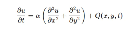
Here, u(x,y,t) is the temperature at a point (x,y) at time t, α is the thermal diffusivity constant, and Q(x,y,t) represents internal heat sources or sinks that can vary in space and time. This PDE is classified as a parabolic equation and typically requires initial and boundary conditions for a complete solution.
In many student assignments or projects, you’ll be working within a rectangular domain—say, simulating heat flow in a room or a metal plate—using either fixed temperatures at boundaries (Dirichlet conditions), insulated edges (Neumann conditions), or a combination of both. Solving this equation over time and space involves discretizing the domain into small cells and advancing the solution forward in time steps using numerical methods.
Discretization: From Continuous to Discrete
The first major step is transforming the continuous equation into a discrete version that MATLAB can handle. This process is called discretization, and it’s typically done using the finite difference method (FDM). For the spatial components, we divide the domain into an N×NN, where each grid point corresponds to a unique temperature value.
Let Δx and Δy represent the grid spacing along the x and y directions, and Δt be the time step size. The second-order spatial derivatives can be approximated using central difference formulas, while the time derivative can be handled with either explicit or implicit schemes. While explicit methods are easy to implement, they are often unstable unless very small time steps are used. For this reason, implicit methods such as backward Euler or Crank-Nicolson are preferred in large and long-time simulations.
Discretizing the 2D heat equation using an implicit method leads to a system of algebraic equations that must be solved at every time step. These systems can become very large, especially when the grid resolution increases, making iterative solvers necessary for efficiency.
The Power of Multigrid Methods
This is where the Multigrid method becomes invaluable. Traditional iterative solvers like Jacobi, Gauss-Seidel, or even Conjugate Gradient can be very slow to converge, especially when the error has low-frequency components. The idea behind multigrid is simple yet powerful: combine fast smoothing methods on fine grids with corrections on coarser grids where low-frequency errors are easier to eliminate.
The Multigrid method works by recursively solving the system at different resolution levels. It includes the following steps:
- Smoothing: Apply a few iterations of a basic solver like Gauss-Seidel to reduce high-frequency errors.
- Restriction: Transfer the residuals to a coarser grid.
- Coarse Grid Correction: Solve the residual equation at the coarser level.
- Prolongation: Interpolate the correction back to the fine grid.
- Update: Adjust the fine grid solution using the interpolated correction.
These steps form a V-cycle or W-cycle pattern depending on the depth of recursion. Because each level of the hierarchy handles different error frequencies, the result is rapid and robust convergence, often independent of grid size.
Implementing the Multigrid Method in MATLAB
A common mistake students make is hardcoding the solution for a single grid size or a specific case. To create a versatile and reusable implementation, one must write modular code that can handle different domain sizes, boundary conditions, and heat source configurations.
First, create a function to generate the coefficient matrix for the discretized 2D Laplacian operator. This matrix depends on the size of the grid and the boundary conditions applied. Next, define a function to perform a single multigrid V-cycle. This function should accept the current guess, the right-hand side, the level of recursion, and the number of pre/post smoothing iterations.
Smoothing can be done using either Gauss-Seidel or weighted Jacobi. For restriction and prolongation, use standard operators such as full-weighting and bilinear interpolation respectively. The coarse grid problem can be solved either directly using matrix inversion (since it’s small) or recursively using another V-cycle.
Handling Heat Sources and Sinks
One often overlooked aspect of heat equation simulations is the inclusion of internal heat generation or absorption. The term Q(x,y,t) allows modeling of real-world scenarios like heaters placed in the room or cooling vents.
In MATLAB, this is implemented as a 2D matrix that matches the domain size. The values in this matrix represent the heat source strength at each point. You can initialize this matrix with zero values and then define specific zones with positive (heat source) or negative (heat sink) values. Make sure that your right-hand side in the discretized system includes this source term properly at each time step.
Students should experiment with both static and time-varying source terms to better understand how heat propagates under different conditions.
Flexible Boundary and Initial Conditions
Another common pitfall is assuming zero Dirichlet boundary conditions. While this may be fine for testing purposes, most realistic simulations require more complex boundaries. For example, walls may be held at a fixed temperature, or some sides may be insulated.
In MATLAB, you should write a boundary handler function that can update the grid values at the edges based on the desired type of boundary. Use logical indexing or loops to apply the boundary conditions before solving the equations in each time
Initial conditions are equally important. These define the temperature distribution at t=0 and should be selected carefully depending on the scenario. You can start with uniform temperature or even apply random distributions to simulate chaotic systems.
Making the Code General and Robust
For your code to be considered robust and suitable for academic evaluation, it must allow changes to problem parameters without breaking. You should be able to change the end time T, the time step Δt, the grid resolution, or even the heat source distribution with minimal code modifications.
To do this, make sure your main solver script accepts input arguments or uses clearly defined parameters at the top of the file. Avoid hardcoded values buried deep in loops or function definitions.
It’s also good practice to test your code against known analytical solutions when available, or to verify convergence by decreasing the grid spacing and observing whether the solution stabilizes.
Demonstrating Multigrid Properties
In academic settings, it’s not enough to just implement the method. You must demonstrate its theoretical benefits with actual results. If you’re claiming faster convergence, provide a comparison of the number of iterations or computation time against Jacobi or Gauss-Seidel methods. If you’re highlighting grid-independent convergence, run the solver on multiple grid sizes and show that the number of V-cycles remains approximately constant.
You should also run your simulation on increasing domain sizes and show that the time complexity grows linearly or nearly linearly, validating the scalability claim of the Multigrid method. For more advanced reports, include contour plots, surface plots, or animated temperature fields over time to showcase how heat propagates under different conditions.
Debugging and Common Pitfalls
Students frequently encounter issues like divergence, incorrect boundary behavior, or runtime errors when increasing grid size or simulation time. These problems usually stem from improper matrix construction, incorrect indexing, or instability in time stepping.
To debug, print intermediate values, visualize the solution at different time steps, and reduce the problem size to isolate issues. Use MATLAB’s built-in visualization tools like imagesc, surf, and contourf to gain insight into your simulation.
Also, always validate your implementation on small domains before scaling up. Use assertions to ensure that matrices have the expected sizes and that residuals are decreasing with each multigrid cycle.
Final Thoughts
Implementing the 2D heat equation using the Multigrid method is both a challenging and rewarding exercise. It offers a deep dive into numerical methods, programming structure, and physical modeling. Students who take the time to build a modular, efficient, and general solver not only complete their assignments successfully but also gain valuable skills applicable to real-world engineering and research problems.
Whether you’re working on a capstone project, coursework, or your own exploration, remember that clarity, flexibility, and validation are key. Don’t just focus on getting the right answer—focus on building a solver that can handle a wide variety of scenarios and back up its results with solid numerical reasoning.
If you need help reviewing your implementation or understanding why a certain aspect isn’t working as expected, use the principles outlined here to guide your debugging and improvement process.