How to Approach MATLAB-Based Control Design Assignments on Multi-Input Single-Output Systems

MATLAB is an essential tool for students, especially when it comes to assignments that require control system simulations, dynamic modeling, and performance analysis. One of the most common types of assignments involves the modeling and simulation of control systems for dynamic systems, such as drones, vehicles, and industrial processes. These types of assignments often require a deep understanding of control theory, system dynamics, and the use of MATLAB for simulation and analysis.
In this blog post, we will walk you through a typical MATLAB assignment that involves control system design for a dynamic system—like a quadrotor drone—but the principles discussed here can be applied to any similar system, whether it's a robot, a vehicle, or a mechanical system with multiple control inputs. This guide will help you solve your Matlab assignment step by step, from the system modeling to the final controller design, providing useful tips and explanations along the way.
Understanding the Problem: System Modeling

Before you start your MATLAB assignment, it's crucial to understand the problem you’re trying to solve. Let’s consider a generic system where you are tasked with controlling a dynamic system that has multiple inputs and outputs. For instance, let's think about a quadrotor drone, where the system’s stability and performance are vital for its safe operation. The drone is equipped with multiple sensors and motors, each contributing to its attitude control, which refers to the aircraft’s orientation in space, including roll, pitch, and yaw rotations.
However, the steps discussed here apply to any dynamic system that requires control design. The process typically involves:
- Defining the system’s transfer functions for each input-output pair (in the case of the drone, these are typically roll, pitch, and yaw control systems).
- Modeling the system dynamics to understand its stability and performance.
- Analyzing the system’s performance through time-domain and frequency-domain responses.
- Designing a controller to ensure that the system meets specific performance criteria, such as rise time, overshoot, and disturbance rejection.
Step 1: Modeling the System in MATLAB
Start by deriving the system's transfer functions, which describe how the inputs (e.g., motor speeds, sensor inputs) affect the system’s outputs (e.g., roll, pitch, yaw angles). In a typical quadrotor system, each motor's dynamics can be represented by transfer functions, such as:
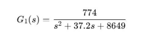
This transfer function represents the relationship between the input (motor input) and the output (angular rotation). If you’re working with a different dynamic system, you'll need to derive the transfer functions based on the system's equations of motion.
Once you have the transfer functions, you can use MATLAB’s built-in functions, such as tf (transfer function) and sys = tf(num, den), to define them in MATLAB.
num = [774];
den = [1, 37.2, 8649];
G1 = tf(num, den);
For more complex systems, you may need to combine multiple transfer functions to form a larger system. MATLAB also allows you to create multi-input, multi-output (MIMO) systems, which is common in drone control design.
Step 2: Block Diagram Reduction and Model Simplification
Once you've defined the transfer functions, the next step is to simplify the system using block diagram reduction techniques. This step is crucial when you're working with systems that have multiple subsystems. For example, in a quadrotor system, you have separate models for roll, pitch, and yaw control, but you need to combine them into a single, simplified model to make the analysis easier.
Manual Approach to Model Reduction
Start by analyzing the system's block diagrams (such as the roll, pitch, and yaw control systems). Use the basic block diagram reduction rules to combine transfer functions and eliminate any redundant components. This can be done manually by following these steps:
- Combine series and parallel systems: For systems in series, simply multiply the transfer functions. For systems in parallel, add the transfer functions together.
- Eliminate feedback loops: Identify feedback loops in the system and simplify them using feedback control techniques. For example, in the roll system, you may have a feedback loop involving the PID controller, which you can reduce.
In MATLAB, you can use feedback or series functions to combine transfer functions. For example:
roll_system = feedback(G1*G2, 1); % Feedback loop for roll control
Using MATLAB for Block Diagram Reduction
Once you've manually reduced the system using block diagram rules, you can verify and finalize the system using MATLAB’s control toolbox. You can represent the reduced system using:
sys_reduced = series(G1, G2); % Combining transfer functions
This way, MATLAB helps you quickly visualize and verify the performance of the reduced system.
Step 3: Dynamic System Analysis
With your reduced system model in hand, the next step is to analyze its dynamics. This step involves plotting the time-domain response (such as the step response) and frequency-domain response (such as Bode and Nyquist plots). These plots help you assess the system's stability and performance.
Time-Domain Analysis: Step Response
The step response of a system shows how the system responds to a sudden change in input. This is particularly useful for analyzing the system's rise time, settling time, and overshoot. To plot the step response in MATLAB, you can use the step function:
step(sys_reduced); % Step response of the reduced system
The step response will provide a visual representation of how the system behaves over time. Key parameters to observe include:
- Rise Time: The time it takes for the system’s output to reach its steady-state value for the first time.
- Settling Time: The time it takes for the system to settle within a certain percentage of its final value.
- Overshoot: The amount by which the system exceeds its final value before settling.
Frequency-Domain Analysis: Bode and Nyquist Plots
Frequency-domain analysis is essential for understanding how the system responds to different frequencies. A Bode plot shows the system's magnitude and phase across a range of frequencies, while the Nyquist plot provides insights into the system’s stability.
To plot the Bode plot in MATLAB, you can use:
bode(sys_reduced); % Bode plot of the reduced system
To plot the Nyquist plot:
nyquist(sys_reduced); % Nyquist plot of the reduced system
From these plots, you can assess the system's stability (e.g., through phase margin and gain margin) and performance (e.g., bandwidth, sensitivity to noise).
Step 4: Controller Design
Now that you've analyzed the system, the next step is controller design. This step involves selecting an appropriate controller to meet the system’s performance specifications. In a typical control system design for a dynamic system like a quadrotor, you may use a PID (Proportional-Integral-Derivative) controller, or more advanced controllers like lead-lag or state-space controllers.
PID Controller Design
A PID controller is commonly used in many control systems due to its simplicity and effectiveness. It provides control by adjusting the output based on the error signal, its derivative, and its integral over time.
In MATLAB, you can define a PID controller as follows:
Kp = 1; % Proportional gain
Ki = 0.1; % Integral gain
Kd = 0.5; % Derivative gain
C = pid(Kp, Ki, Kd);
Once you have defined your controller, you can incorporate it into the system using feedback control. For example, to add the PID controller to the roll system:
roll_with_controller = feedback(C * G1, 1); % Closed-loop system with PID
Lead-Lag Compensator Design
For more advanced systems or when the performance requirements are stricter, you might choose to use a lead or lag compensator. A lead compensator is used to increase the system's phase margin and improve stability, while a lag compensator can improve steady-state accuracy.
In MATLAB, you can define a lead compensator as:
K = 10; % Gain for lead compensator
alpha = 1.5; % Lead compensator parameter
lead_compensator = K * (s + alpha) / (s + 1);
Step 5: Performance and Stability Evaluation
Once you’ve implemented the controller, it’s time to evaluate the system’s performance and stability. This step involves checking if the system meets the desired specifications for rise time, overshoot, settling time, and disturbance rejection.
In MATLAB, you can assess the disturbance rejection by introducing a disturbance signal into the system. For instance, you can use the following command to simulate a disturbance and analyze its impact:
disturbance = 0.1 * sin(0.1 * t); % Disturbance signal
Then, you can assess how well the system rejects the disturbance by plotting the system’s response with and without the disturbance.
Conclusion:
Solving a MATLAB control system assignment requires several key steps: modeling the system, reducing the block diagram, analyzing its dynamics, designing a suitable controller, and evaluating its performance and stability. By following this step-by-step process, you can approach any MATLAB assignment with confidence and ensure that your solutions meet the required specifications.
Whether you're working on a quadrotor drone, a robotic arm, or another type of dynamic system, the principles discussed here apply universally. The key is to use MATLAB’s powerful tools to model, simulate, and optimize your system effectively. Remember to always verify your results through different analyses and ensure that the final system performs as required.
By following these guidelines, you can successfully tackle MATLAB assignments and gain valuable insights into control systems, which are applicable to real-world engineering problems.