How to Effectively Handle MATLAB Assignment on Fourier Series

Fourier Series is an essential tool in signal processing, widely used to analyze and approximate periodic signals. MATLAB, a powerful computational software, is perfect for calculating and visualizing Fourier Series. Whether you're working with simple periodic signals like square waves or more complex functions, MATLAB offers an intuitive approach to understanding and implementing the Fourier Series.
This blog post aims to guide you through the process of solving Fourier Series problems in MATLAB. While we won’t be focusing on any specific problem, this comprehensive guide will provide you with the essential steps to solve your matlab assignment related to Fourier Series calculations, helping you better understand the underlying mathematics and its implementation.
What is the Fourier Series?

Before diving into the MATLAB implementation, it is essential to understand what the Fourier Series is and how it is used. The Fourier Series represents a periodic function as a sum of sine and cosine terms. Essentially, it decomposes any periodic signal into a series of harmonics, each contributing to the overall waveform.
The general form of the Fourier Series expansion for a periodic function f(t) with period T is:
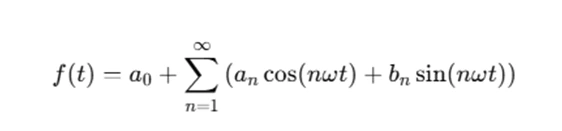
Where:
- a0 is the DC component or the average value of the signal.
- ana and bnb are the Fourier coefficients for the cosine and sine terms, respectively.
- n represents the harmonic number.
- ω=2πT is the angular frequency of the signal.
These coefficients, a0, ana, and bnb, are calculated by integrating the function over one period.
Step 1: Understanding the Problem
To solve your Fourier Series assignment problem in MATLAB, you first need to understand the problem you're working on. Typically, you are asked to calculate the Fourier Series for a specific signal. Let’s take an example of a square wave function. You might be given an amplitude A and a vector H representing the harmonics you need to use in the Fourier Series calculation.
The signal is defined as a square wave, where the function takes values of A in the interval [−0.5,0.5] and 0 elsewhere. The Fourier Series approximation for this signal will involve calculating the Fourier coefficients for the specified harmonics and comparing the approximation to the original signal.
Defining the Inputs:
The key inputs for your MATLAB function will include:
- Amplitude A: This defines the peak value of your signal.
- Harmonics H: A vector of harmonic numbers that specifies how many terms you want to include in your Fourier Series approximation. The length of this vector will determine how many times the function is iterated, allowing you to calculate the Fourier Series for different numbers of harmonics.
For instance, if H=[1,3,5], your function will calculate the Fourier Series three times:
- Once with the fundamental frequency and the first harmonic.
- Once with the fundamental frequency and the first three harmonics.
- Once with the fundamental frequency and the first five harmonics.
Understanding the Symbolic Approach:
The key to solving Fourier Series problems in MATLAB is using symbolic computation. MATLAB’s symbolic toolbox allows you to work with symbolic expressions, making it easier to calculate the Fourier coefficients. Instead of solving the integrals numerically, you can use the syms function to create symbolic variables and then compute the coefficients symbolically.
For example, to represent a square wave function in MATLAB, you can use the heaviside function:
syms t
f_t = A * (heaviside(t + 0.5) - heaviside(t - 0.5));
This defines the square wave f(t) with amplitude A. The heaviside function is a standard way to represent step functions, which is what a square wave consists of.
Step 2: Calculate Fourier Coefficients
To calculate the Fourier Series, the next step is to compute the Fourier coefficients a0, ana, and bnb. These coefficients are determined through integration over one period of the signal.
The formula for these coefficients are:
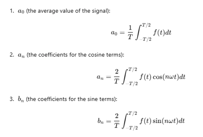
In MATLAB, you can calculate these integrals symbolically. For instance, to compute ana and bnb, you can use the int function to integrate the symbolic expression f(t) with the corresponding sine or cosine function:
a_n = int(f_t * cos(n * omega * t), t, -T/2, T/2);
b_n = int(f_t * sin(n * omega * t), t, -T/2, T/2);
Step 3: Reconstruct the Fourier Series
Once you have the Fourier coefficients, you can reconstruct the Fourier Series for each harmonic specified in the vector H. The Fourier Series is given by:
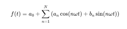
Where N is the maximum harmonic number you are considering. You will loop over the elements of H and calculate the Fourier Series for each corresponding harmonic count.
FS = a_0 + sum(an .* cos(H .* t) + bn .* sin(H .* t), 2);
Step 4: Visualizing the Signal and Fourier Series
One of the most useful features of MATLAB is its ability to plot data. After computing the Fourier Series, you can compare the original signal and the Fourier Series approximation visually. To do this, you need to plot the original signal and the Fourier Series approximation on the same graph.
Start by defining a time vector that spans one period of the signal. For example, you can create a time vector from t=−1 to t=1 with a sufficiently high resolution:
t = linspace(-1, 1, 1000);
Now, you can compute the original square wave signal and the Fourier Series approximation:
f_original = A * (heaviside(t + 0.5) - heaviside(t - 0.5));
f_approx = a0 + sum(an .* cos(H .* t) + bn .* sin(H .* t), 2);
Finally, plot the original signal and the Fourier Series approximation:
figure;
plot(t, f_original, 'b', t, f_approx, 'r');
legend('Original Signal', 'Fourier Approximation');
This will display the original signal in blue and the Fourier Series approximation in red.
Step 5: Calculate the Error (SSE)
To assess the quality of the Fourier Series approximation, you can calculate the error between the original signal and the approximation. The error is typically measured using the Sum of Squared Errors (SSE), defined as:
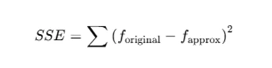
In MATLAB, this can be computed easily:
SSE = sum((f_original - f_approx).^2);
This gives you a numerical measure of how well your Fourier Series approximation fits the original signal. The SSE will decrease as you include more harmonics in the Fourier Series.
Step 6: Loop Through Multiple Harmonics
In many Fourier Series problems, you need to calculate the Fourier Series for different numbers of harmonics. This is where MATLAB’s for loop comes in handy. You can loop through the harmonics specified in the vector H and compute the Fourier Series approximation for each set of harmonics.
Here’s how you might loop through the harmonics:
for n = 1:length(H)
    harmonics = H(n);
    % Calculate Fourier coefficients and approximation for each harmonic
    % Plot results
End
For each iteration, you can calculate the Fourier coefficients ana, bnb, and reconstruct the Fourier Series, then plot the results in a new subplot.
Step 7: Plot the Error vs. Number of Harmonics
Another useful visualization is to plot the SSE as a function of the number of harmonics. This helps to demonstrate how the approximation improves as you include more harmonics.
Here’s how you can plot the SSE vs. the number of harmonics:
SSE_values = [];
for n = 1:20
    % Compute Fourier Series approximation for n harmonics
    % Calculate the SSE
    SSE_values(end+1) = SSE;
end

% Plot SSE vs Number of Harmonics
figure;
plot(1:20, SSE_values);
xlabel('Number of Harmonics');
ylabel('SSE');
title('Error vs Number of Harmonics');
Conclusion
In this blog, we have outlined the essential steps to solve Fourier Series problems in MATLAB. By following these steps, you will be able to calculate the Fourier Series for any periodic signal, whether it is a square wave, sawtooth wave, or any other signal.
The process includes defining the signal, calculating the Fourier coefficients, reconstructing the Fourier Series, and visualizing the results. Moreover, by calculating the error (SSE), you can evaluate how well your Fourier Series approximation matches the original signal.
By practicing these steps and experimenting with different signals and numbers of harmonics, you’ll improve your understanding of both Fourier Series and MATLAB.