Mastering 3D Two-Phase Flow Simulations in MATLAB: A Comprehensive Guide

3D two-phase flow simulation is a pivotal component in reservoir engineering, facilitating the understanding of fluid dynamics within reservoirs. This guide aims to provide a structured methodology for developing a numerical simulator for two-phase gas-water flow using MATLAB, applicable to various assignments and projects. By adhering to this guide, you will be equipped to solve your MATLAB assignment efficiently and accurately.
Understanding the Problem
Before embarking on the coding journey, it is crucial to fully grasp the problem at hand. The primary objective is to develop a numerical simulator for two-phase gas-water flow in reservoirs using a fully implicit method. The project involves addressing partial differential equations (PDEs) that describe fluid flow, deriving finite difference equations, implementing and validating the simulator with water flooding scenarios, and generating comprehensive results.
Step-by-Step Approach

Step 1: Define the Governing Equations
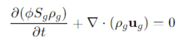
Fluid flow in reservoirs is governed by the continuity equations for each phase and Darcy’s law. The general partial differential equations (PDEs) for two-phase (gas and water) flow can be represented as follows:
Gas Phase:
Water Phase:
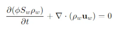
Here, ϕ\phiϕ represents porosity, SgS_gSg and SwS_wSw are saturations, ρg\rho_gρg and ρw\rho_wρw are densities, and ug\mathbf{u}_gug and uw\mathbf{u}_wuw are velocities for gas and water phases, respectively.
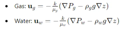
Darcy's law for each phase is given by:
Step 2: Discretize the Equations
Using finite difference methods, the PDEs are discretized over a grid. For a 3D grid, this involves spatial (x, y, z) and temporal (t) steps.
An example of a finite difference approximation for the pressure equation is:
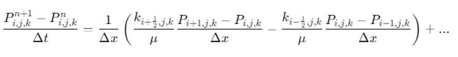
This discretization converts the PDEs into a system of algebraic equations that can be solved iteratively.
Step 3: Implement the Simulator in MATLAB
- Initialize Parameters: Set up the initial conditions, reservoir properties, and simulation parameters.
- Grid Setup: Define the grid dimensions and allocate memory for pressure, saturation, and other variables.
- Time Loop: Implement the time-stepping loop where, at each step, pressures and saturations are updated, boundary conditions are applied, and the linear system of equations is solved using iterative solvers like Gauss-Seidel or Conjugate Gradient.
Example Code Structure:
% Initialize parameters
Nx = 50; Ny = 50; Nz = 10; % Grid dimensions
dx = 20; dy = 20; dz = 5; % Grid spacing
T = 365; % Simulation time in days
dt = 1; % Time step in days
% Initialize variables
P = ones(Nx, Ny, Nz) * 3000; % Initial pressure
Sw = ones(Nx, Ny, Nz) * 0.3; % Initial water saturation
% Time loop
for t = 1:dt:T
% Update pressures and saturations
for i = 2:Nx-1
for j = 2:Ny-1
for k = 2:Nz-1
% Apply finite difference approximations
% Update P and Sw based on discretized equations
end
end
end
% Apply boundary conditions
% ...
% Solve linear system
% ...
End
Step 4: Validate and Analyze Results
Once the simulator is implemented, it’s essential to validate the results by comparing them with known solutions or analytical results. The following outputs are typically required:
1. Pressure and Saturation Maps: Generate maps at specified intervals using MATLAB plotting functions. These maps visualize the spatial distribution of pressure and saturation within the reservoir over time.
% Plot pressure map
figure;
imagesc(P(:,:,5)); % Example slice at mid-depth
title('Pressure Map');
colorbar;
2. Production Rates: Calculate and plot gas and water production rates over time. These plots help in understanding the performance of the reservoir under different flooding scenarios.
% Calculate production rates
gas_production_rate = ...; % Compute based on updated variables
water_production_rate = ...; % Compute based on updated variables
% Plot production rates
figure;
plot(time, gas_production_rate, 'r', time, water_production_rate, 'b');
legend('Gas', 'Water');
title('Production Rates');
xlabel('Time (days)');
ylabel('Production Rate (bbl/day)');
By following these steps, you can develop a robust 3D two-phase flow simulator in MATLAB. This guide provides a structured approach that can be adapted to various similar assignments, ensuring you cover all necessary aspects from understanding the problem, discretizing equations, coding, and validating results.
Additional Considerations
Numerical Stability and Convergence
Ensuring numerical stability and convergence is crucial in simulation projects. Here are a few tips:
- Time Step Size: Choose an appropriate time step size. Too large a time step can lead to instability, while too small a time step can increase computational load.
- Grid Resolution: Ensure that the grid resolution is fine enough to capture essential details but coarse enough to remain computationally feasible.
- Solver Selection: Select an efficient solver that ensures rapid convergence. Iterative solvers like Conjugate Gradient or BiCGSTAB are often preferred for large systems.
Boundary Conditions
Applying correct boundary conditions is critical. For a closed reservoir:
- No-flow boundary conditions should be applied at the edges.
- For partially penetrated wells, specify the appropriate penetration depth and apply the conditions only within that segment.
Handling Nonlinearities
Nonlinearities can arise from various factors, including fluid properties and relative permeabilities. Implementing a robust method to handle these nonlinearities, such as Newton-Raphson, can significantly enhance the simulator's accuracy.
Conclusion:
Developing a 3D two-phase flow simulator requires a blend of theoretical understanding and practical implementation skills. By mastering these techniques and utilizing the resources available, you will be well-equipped to tackle complex reservoir simulation projects in both academic and professional settings.
Additional Resources
To further enhance your understanding and capabilities, consider the following resources:
- MATLAB Documentation: Essential for understanding MATLAB functions and capabilities.
- Textbooks: "Applied Petroleum Reservoir Engineering" by B.C. Craft and M.F. Hawkins offers foundational knowledge.
- Research Papers: Explore advanced methods and case studies to broaden your knowledge.
By systematically applying the principles outlined in this guide, you can confidently approach and solve 3D two-phase flow simulation assignments in MATLAB, ensuring both accuracy and efficiency in your results.