Effective Methods for Solving MATLAB Assignments on Fluid Flow Simulation

When dealing with complex engineering problems like single-phase gas flow in reservoirs, students often struggle to apply theoretical concepts to real-world scenarios. One such task is creating a reservoir simulator for single-phase gas flow, which requires translating mathematical models into practical simulations. Typically, this involves choosing between a 1D, 2D, or 3D model to accurately represent how fluid moves through a reservoir. These models require students to understand and solve partial differential equations that describe fluid dynamics, considering factors like permeability, pressure, and rock compressibility. The goal is to simulate the gas flow behavior over time, helping engineers predict production rates and pressure distributions. With the right approach and tools, students can break down this complex assignment into manageable steps, ultimately creating a functional simulator that offers valuable insights into reservoir behavior and gas extraction processes. This guide will provide an outline for solving assignments similar to those in gas reservoir simulation and offer step-by-step instructions to help with fluid dynamics simulations assignment and navigate similar tasks efficiently.

Understanding to Reservoir Simulation
Reservoir simulation is a crucial technique used in petroleum engineering to predict the behavior of fluids (like gas or oil) in underground reservoirs. In a gas reservoir, understanding how the gas behaves as it moves through porous rock layers is vital for optimal production strategies. For this type of assignment, you may be tasked with building a simulator that computes gas production rates, pressure distributions, and other reservoir properties under certain conditions.
The following sections will guide you through the general process of solving assignments of this nature, which may involve constructing partial differential equations, solving them with numerical methods like Finite Difference, and interpreting the results for meaningful insights.
Step 1: Understanding the Governing Equations
The first step in any simulation task is to understand the governing equations. For gas flow in reservoirs, the fundamental equation is a form of the diffusion equation, often expressed as a partial differential equation (PDE). In the case of a single-phase gas reservoir simulator, the equation takes into account various factors like pressure, permeability, porosity, and compressibility.
For example, a general equation for gas flow in porous media can be expressed as:
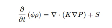
Where:
- ϕ is the porosity,
- ρ is the gas density,
- K is the permeability,
- P is the pressure,
- S represents the source term (like the injection or production of gas).
These equations are typically solved numerically because an analytical solution is often too complex for realistic reservoir configurations. The next task is discretizing the equation using methods like the Finite Difference method (FDM).
Step 2: Deriving Finite Difference Equations
Finite difference methods are widely used to solve PDEs numerically. The idea behind FDM is to approximate derivatives using differences between function values at discrete points.
For a 1D example, the general approach would be to discretize the spatial and temporal derivatives. Let’s consider the following equation for 1D gas flow:
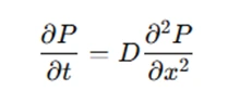
Where D is a diffusion coefficient. To discretize this equation using finite differences, we replace the spatial and time derivatives with finite difference approximations.
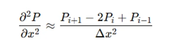
For example, for the spatial derivative, we can use the central difference approximation:
For the time derivative, a forward difference scheme can be used:
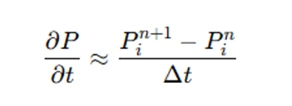
This results in a finite difference equation that updates the pressure values at each time step:
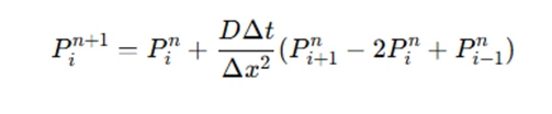
This equation can be extended to 2D or 3D problems by incorporating additional spatial dimensions and updating the pressure at each point in the grid.
Step 3: Implementing the Numerical Solution
Once the finite difference equations are derived, the next step is to implement the solution numerically. This is typically done by writing code in MATLAB or similar programming languages. Below is an example of MATLAB code that implements the 1D finite difference method for the gas flow equation.
% Parameters
L = 1000;  % Length of the reservoir (m)
T = 1000;  % Total simulation time (s)
Nx = 50;   % Number of spatial points
Nt = 200;  % Number of time steps
dx = L / (Nx-1);  % Spatial step
dt = T / Nt;      % Time step
D = 1e-5;         % Diffusion coefficient (m^2/s)

% Initial condition
P = zeros(Nx, Nt);  % Pressure matrix
P(:, 1) = 3000;      % Initial pressure in all points (psia)

% Finite difference loop
for t = 1:Nt-1
    for x = 2:Nx-1
        P(x, t+1) = P(x, t) + (D * dt / dx^2) * (P(x+1, t) - 2*P(x, t) + P(x-1, t));
    end
end

% Plot the results
time = linspace(0, T, Nt);
plot(time, P(round(Nx/2), :));
xlabel('Time (days)');
ylabel('Pressure (psia)');
title('Pressure vs Time at the Reservoir Center');
In this code, we create a 1D grid with a set number of spatial points and time steps. The code then iterates over the grid, applying the finite difference scheme to update the pressure values. The final result is a plot showing the pressure evolution over time at the center of the reservoir.
Step 4: Analyzing the Results
Once the simulation is complete, it's time to analyze the results. The results usually include:
- Gas Production Rate vs. Time: This is a graph that shows how the production rate of gas evolves over time. You can compute this from the pressure difference between the production well and the surrounding reservoir using a well model.
- Pressure Distribution at Different Times: The pressure distribution within the reservoir can be plotted at specific time intervals (e.g., 5, 10, 20, and 30 days). This provides insight into how pressure declines as gas is produced from the reservoir.
For example, you can use the following code snippet to plot the pressure distribution at specific time steps:
% Plot pressure distribution at specific times
time_steps = [5, 10, 20, 30];  % Times to plot (in days)
for i = 1:length(time_steps)
    t_index = round(time_steps(i) * Nt / T);
    plot(linspace(0, L, Nx), P(:, t_index));
    hold on;
end
xlabel('Distance (m)');
ylabel('Pressure (psia)');
title('Pressure Distribution at Different Times');
legend('5 days', '10 days', '20 days', '30 days');
This code will generate a plot showing the pressure profiles at various time intervals, helping you visualize how pressure changes over the course of the simulation.
Step 5: Verifying Results and Debugging
After obtaining results from a MATLAB simulation, it’s crucial to verify their accuracy. Sometimes, the solution may not converge, or the results may deviate from expectations. This could be due to several factors, such as incorrect boundary conditions, inappropriate model assumptions, or numerical instability. To ensure reliability, it's important to cross-check the results with analytical solutions or known benchmarks. If discrepancies arise, adjusting the model parameters, refining the grid resolution, or using different numerical methods, such as the fully implicit method, can help improve convergence and result accuracy. Common issues include:
- Convergence Issues: If the solution does not converge, consider reducing the time step or checking the boundary conditions.
- Incorrect Initial Conditions: Ensure that the initial pressure and other parameters are set correctly according to the problem statement.
Always verify the physical relevance of your results. If the results seem unrealistic, retrace your steps and check your code for errors.
Conclusion
In summary, solving a single-phase gas flow simulator assignment involves a clear understanding of the governing equations, discretizing them using finite difference methods, implementing the numerical solution in MATLAB, and interpreting the results. By following this structured approach, students can successfully complete their MATLAB assignment while gaining a deeper understanding of reservoir simulation techniques.
With the right tools and strategies, solving similar fluid dynamic simulation assignments becomes a manageable task. Whether working on gas flow simulation, oil reservoir modeling, or similar engineering problems, the steps outlined in this guide will serve as a strong foundation for successfully tackling complex simulation challenges.