How to Approach Complex Electromagnetism Assignments Using MATLAB

Electromagnetic theory forms the bedrock of modern physics and electrical engineering, and understanding it can be challenging for many students. One key to mastering electromagnetism is developing a structured approach to solve problems—especially those that involve Maxwell's equations, material properties like permittivity, and simulation tools like MATLAB. This blog is aimed at guiding students through these complex topics, offering practical advice on how to solve their Matlab assignment on electromagnetic effectively. Whether you're dealing with static or dynamic cases, this guide will equip you with the skills to navigate through your assignments with confidence.
1. Mastering the Fundamentals: Maxwell's Equations
Maxwell’s equations are the foundation of electromagnetism. They describe how electric and magnetic fields interact, and they are essential for understanding how materials respond to electromagnetic fields. Here’s a quick overview of the four Maxwell equations that are vital for solving many physics and engineering problems:

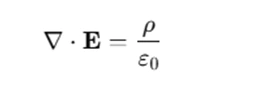
Gauss's Law for Electricity
Gauss’s law relates the electric field to the distribution of electric charges. It states that the electric flux through any closed surface is proportional to the charge enclosed within the surface.
Where:
- E is the electric field,
- ρ is the charge density,
- ε0 is the permittivity of free space.
Gauss's Law for Magnetism
Gauss’s law for magnetism states that magnetic monopoles do not exist, and the magnetic field lines form continuous loops.
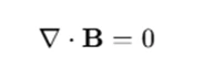
Where:
- B is the magnetic field.
Faraday’s Law of Induction
Faraday’s law shows how a time-varying magnetic field generates an electric field.

Where:
- ∇×E is the curl of the electric field,
- ∂B/∂t is the time rate of change of the magnetic field.
Ampère's Law with Maxwell’s Addition
Ampère's law describes how electric currents and changing electric fields produce magnetic fields.
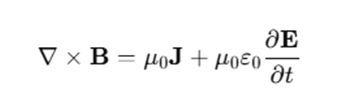
Where:
- J is the current density,
- μ0 is the permeability of free space.
2. Approaching the Derivation Process
A common theme in electromagnetism assignments is the need to derive relations based on Maxwell’s equations and material properties like permittivity and permeability. Here’s how you can break down complex derivations:
Identifying the Parameters
The first step in any problem is to carefully read the given information. Identify the key parameters—whether they are constants (e.g., permittivity ε0, permeability μ0) or variables related to the material properties (e.g., the polarization P, the displacement field D).
Starting from Basic Assumptions
Many electromagnetism problems assume that the material under consideration is a dielectric (non-conducting material). For example, in the case of static permittivity, you might assume that the material's atoms or molecules induce dipole moments when exposed to an electric field.
You might start by deriving the relationship between electric displacement field (D), electric field (E), and polarization (P):

Where:
P is the polarization vector, which describes the material's response to the electric field.
This is a crucial step when deriving equations for static and dynamic permittivity.
Introducing Material Effects
In many cases, the material properties like permittivity and permeability affect how electric and magnetic fields propagate. For instance, the static permittivity ε for a material is typically defined as:
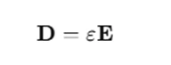
The constitutive relation helps to express how the material modifies the electric field and magnetic field in its presence.
3. Understanding the Vector Fields: P and D
In electromagnetism, the vector fields P (polarization) and D (electric displacement) are crucial for understanding the material response to electric fields.
The Vector Field P\mathbf{P}P
The polarization vector P represents the dipole moment per unit volume of a dielectric material. When an external electric field is applied to the material, it induces alignment in the molecules, creating a net dipole moment. This polarization describes how the material responds to the electric field.
The Vector Field D\mathbf{D}D
The displacement field D incorporates both the effects of free charges and bound charges within the material. It helps simplify Maxwell’s equations in materials and allows for a unified description of the material's response to an electric field. The electric displacement field is defined as:

The Role of D\mathbf{D}D
The vector field D plays a critical role in understanding the macroscopic response of materials to external electric fields. It helps to distinguish between free and bound charges in the material and allows us to solve problems without needing to consider polarization effects separately.
4. Dynamic Problems: A.C. Permittivity and the Lorentz Model
In dynamic cases, where the electric field is oscillating or varying with time, the material's response changes. This requires the use of more advanced models like the Lorentz model, which explains the behavior of atoms under oscillating electric fields.
Mechanical Analogy for Polarized Atoms
To understand the behavior of materials under time-varying fields, start with the mechanical analogy of an atom under an oscillating electric field. Imagine an electron bound to a nucleus by a restoring force (much like a spring). When an oscillating electric field is applied, the electron oscillates, leading to a polarization of the atom.
Deriving the Lorentz Model
The Lorentz model describes how this polarization evolves over time when the material is exposed to a time-varying electric field. From this, we can derive the dispersion relation, which describes how the material’s permittivity changes with frequency. The key here is understanding the relationship between the material’s microscopic behavior (e.g., electron motion) and its macroscopic properties (e.g., permittivity).
5. Using MATLAB for Simulations and Plots
Once you’ve derived the theoretical equations, the next step is to simulate and visualize the results using MATLAB. MATLAB is an essential tool for solving complex electromagnetic problems and visualizing the behavior of materials under different conditions.
Setting Up the Parameters
Before you can start plotting, you need to define the physical parameters in MATLAB. For example, define values for the frequency, permittivity, and other material constants. A typical MATLAB code block might look like this:
w0 = 7; % Frequency
alpha = 1.1;
m = 1;
Eom = 3;
% Define material properties and other parameters
Implementing the Dispersion Relation
Once you’ve set up the parameters, the next step is to implement the dispersion relation for permittivity. This can be done by writing functions or scripts that calculate the permittivity at different frequencies and then plotting the results. Use functions like plot or mesh to visualize how the permittivity changes over time or frequency.
Plotting the Results
MATLAB’s plotting functions are incredibly useful for visualizing how material properties behave under different conditions. For example, you might plot the dispersion relation to see how permittivity changes as a function of frequency.
% Example of plotting the dispersion relation
plot(frequency, permittivity)
title('Dispersion Relation')
xlabel('Frequency (Hz)')
ylabel('Permittivity')
6. Key Models to Know: Drude and Clausius-Mossotti
Two other important models that often appear in assignments are the Drude model and the Clausius-Mossotti formula.
The Drude Model
The Drude model explains how free electrons in metals respond to electric fields. It starts from the Lorentz model but incorporates the behavior of free electrons in a conducting material. The Drude dispersion function is a critical tool in understanding how materials like metals behave under electromagnetic waves.
To solve assignments involving the Drude model, derive the model’s equations based on the material’s properties and then use MATLAB to plot the dispersion function. For example, using the Drude parameters for silver (Ag), you can plot the material’s permittivity as a function of frequency and discuss the implications of the plasma frequency.
Clausius-Mossotti Formula
The Clausius-Mossotti formula relates the macroscopic permittivity of a material to its microscopic properties. It can be used to calculate the relative permittivity of materials, such as a cubical lattice of conducting spheres. By following the derivation in your course notes, you can use the formula to calculate the material’s relative permittivity and compare it to other materials.
7. General Tips for Tackling Electromagnetic Assignments
Here are some tips that can help you approach electromagnetism assignments effectively:
- Break Down the Problem Step by Step
- Use Physical Intuition
- Verify Your Results
- Ask for Help
Electromagnetic problems can often seem overwhelming at first, but breaking them down into smaller, manageable steps makes the process much easier. Start from basic principles and work your way through the derivations logically.
Don’t just rely on equations—try to develop an intuitive understanding of the physical phenomena at play. For example, understanding the meaning behind terms like permittivity and polarization can help guide you through the derivations and make sense of the results.
Whenever possible, compare your MATLAB results with theoretical predictions or known results from textbooks. This will help you catch any mistakes early and ensure your approach is on the right track.
If you’re stuck, don’t hesitate to ask for help. Consult your textbooks, professors, or online forums. Sometimes, a small hint or clarification can make a huge difference in solving a complex problem.
Conclusion
Mastering electromagnetism requires a deep understanding of theoretical concepts along with practical skills in simulation and visualization. By approaching problems methodically—starting from foundational principles—and leveraging tools like MATLAB for simulations, you can tackle even the most complex assignments. MATLAB helps visualize electromagnetic phenomena, simplifying the learning process. With consistent practice, you’ll gain confidence in applying Maxwell's equations and material properties to real-world scenarios. This combination of theory and hands-on problem-solving will make electromagnetism not only more approachable but also a highly rewarding subject to study and apply in various fields of science and engineering.