How to Solve Amplitude Modulation Assignments using MATLAB

In signal processing courses, assignments involving Amplitude Modulation (AM), Fourier Transforms, and system analysis. Successfully tackling these tasks requires both theoretical knowledge and practical MATLAB programming skills. In this blog, we will outline a structured approach how to solve their Matlab assignment AM-based, helping you break them down into manageable steps.
A typical AM assignment requires understanding how a message signal is modulated, analyzing its frequency components, and using MATLAB to process signals. Start by loading the given dataset, which may include modulation frequencies, filter coefficients, and signal waveforms. Next, visualize key components like Morse code signals or modulation waveforms using plots. Analyzing the frequency response of filters and signal transformations using Fourier analysis is crucial for extracting meaningful information.

MATLAB functions such as freqs(), fft(), and lsim() help in analyzing signal behavior. You may also need to reconstruct signals from given components or determine unknown parameters. By systematically approaching each task—loading data, visualizing signals, applying transformations, and interpreting results—you can confidently tackle AM-based assignments. While each assignment varies, following this structured method ensures an effective problem-solving approach, improving both your understanding and MATLAB proficiency.
1. Understand the Problem Statement
Before starting in MATLAB, it's crucial to understand the assignment requirements. For example, if you're working with an amplitude modulation (AM) system, you must grasp how a message signal is modulated onto a carrier wave. This involves analyzing the given mathematical expressions, understanding the role of modulation frequencies, and interpreting how signals are represented. Additionally, familiarize yourself with provided data files, such as time samples and filter coefficients, to ensure proper signal processing. A solid conceptual foundation will help you efficiently implement the necessary MATLAB functions and extract meaningful insights from the given signal data. A typical AM signal is represented as:
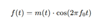
Here, m(t)m(t)m(t) is the message signal, and f0f_0f0 is the modulation frequency. By understanding the mathematical relationships in the problem, you'll be better equipped to translate these concepts into MATLAB code.
2. Load the Data and Preprocessing
Many assignments include preloaded datasets or signal files, such as data.mat, which provide essential information for signal processing tasks. These files typically contain message signals, modulation frequencies, filter coefficients, and sequences like dash and dot signals used in Morse code. Students must analyze and manipulate these signals to extract meaningful information, such as identifying encoded messages or filtering noise. Understanding how to load, visualize, and process these datasets is crucial for solving assignments effectively. By mastering these fundamental techniques, students can confidently approach similar problems in amplitude modulation, Fourier analysis, and signal decomposition in various applications. The first step in MATLAB is to load these datasets and take a look at the variables:
load('data.mat'); % Load the data file
You’ll likely encounter variables like x(t), which contains the AM signal, dash and dot signals for Morse code representation, or filter coefficients. Always check the variables in the workspace using whos to see what you’re working with.
3. Plotting and Visualizing Signals
Visualizing signals through plotting is essential for analyzing their properties and behavior. It helps in identifying patterns, understanding frequency components, and verifying signal processing steps. Proper signal representation through graphs aids in troubleshooting, ensuring accuracy, and interpreting results effectively in assignments related to amplitude modulation and Fourier analysis. For example, you may be asked to plot the dash and dot signals used to represent Morse code:
plot(t, dash); % Plot the dash signal
xlabel('Time (s)');
ylabel('Amplitude');
title('Dash Signal');
grid on;
Additionally, if the assignment involves a specific filter, you may need to visualize its frequency response to understand its behavior. Use freqs to plot the frequency response of the low-pass filter:
freqs(bf, af); % Plot the filter's frequency response
4. Signal Modulation and Filtering
Many assignments involve studying modulation techniques like amplitude and frequency modulation. These concepts help in signal processing, communication systems, and data transmission. Understanding how modulation alters signals enables students to analyze and decode waveforms effectively. Mastering these techniques is essential for applications in wireless communication, broadcasting, and digital signal processing. You will likely need to create a modulated signal by multiplying the message signal with a cosine or sine function. For example:
y = dash .* cos(2 * pi * f1 * t); % Modulate the dash signal
After modulation, filtering may be required. Use lsim to apply the filter to your modulated signal:
y_filtered = lsim(bf, af, y, t);
Once filtered, plot the original and filtered signals side by side to compare:
subplot(2,1,1);
plot(t, y);  % Plot original modulated signal
title('Original Modulated Signal');
subplot(2,1,2);
plot(t, y_filtered);  % Plot filtered signal
title('Filtered Signal');
5. Fourier Transform Analysis
A key to solving such problems is understanding signal behavior in the frequency domain. The Fourier transform helps analyze how signal components are distributed across frequencies. This is crucial for tasks like extracting modulated signals, filtering, and interpreting results in amplitude modulation systems, ensuring accurate signal processing and decoding. To find the Fourier transform of the modulated signal, use MATLAB’s fft function:
FT_y = fftshift(fft(y));
L = length(y);
Fs = ceil(1/t(2));  % Sampling frequency
w = 2 * pi * Fs * (-L/2 : L/2-1) / (L-1);
plot(w, abs(FT_y));
title('Spectrum of Modulated Signal');
xlabel('\omega (rad/sec)');
grid on;
6. Signal Demodulation
In tasks where you need to extract modulated signals, such as the four-letter Morse code word encoded in your signal, demodulation becomes essential. You’ll have to apply techniques like low-pass filtering and peak detection to extract the original message. Use MATLAB to perform the demodulation process:
% Demodulate signal
y_demodulated = y_filtered .* cos(2 * pi * f1 * t);
To identify the individual Morse code letters, you may need to identify patterns in the signal (e.g., periods of silence and bursts corresponding to dots and dashes) and match these to the Morse code chart.
7. Understanding Frequency Components
Another critical aspect of these assignments is understanding how the signal's frequency components interact with the filter’s passband. You’ll need to perform analysis by looking at the frequency components of your dash and dot signals:
ydash = lsim(bf, af, dash, t(1:length(dash)));
ydot = lsim(bf, af, dot, t(1:length(dot)));
Then, visualize both the original and filtered signals to see how the filter affects different frequency components.
8. Extracting Information from the Signal
After completing the required processing and visualizations, the next step is extracting meaningful information from the signal. This involves analyzing the modulated signal, identifying frequency components, and applying filtering techniques to isolate relevant waveforms. By interpreting the Fourier transform results and the lowpass filter’s response, you can decode embedded signals, such as Morse code letters. Proper extraction ensures accurate identification of underlying patterns in the data. This process is crucial in signal analysis, helping to reconstruct original messages or detect specific elements within a complex waveform, leading to a deeper understanding of the given signal’s characteristics. For example, if you’re working with Morse code, extract the individual letters encoded in the modulated signal and use the Morse code chart to identify the message.
% Use time-domain analysis or pattern recognition to decode Morse
letters = decodeMorse(ydash, ydot);  % Hypothetical decoding function
Conclusion
By following these steps, students can approach their AM modulation assignments in MATLAB with confidence. Whether working with low-pass filters, performing Fourier analysis, or decoding Morse code messages, understanding the underlying signal processing principles and mastering the necessary MATLAB functions are key to solving these assignments successfully. Remember, each assignment may have its own specific requirements, but the fundamental concepts will remain the same.
If you ever find yourself struggling, remember that it’s always a good idea to break the problem down into smaller tasks, plot your signals at every step, and understand the underlying theory behind each operation. This method will not only help you complete your signal processing assignment and solidify your understanding of techniques.